4 Data Frames
We have used information about a 14-member family to demonstrate several features of the R language. This information appears in several vectors, each with 14 elements. It’s natural for us to picture this information arranged in a table, where each column of the table corresponds to a variable, like name, age, height and weight, and each row corresponds to a particular individual, such as the 77-year old named Tom in the first row and the 27 year-old named Sue in the 5th row. R provides a data structure, called a data frame, for collecting vectors into one object, which we can imagine as a table. More specifically, a data frame is an ordered collection of vectors, where the vectors must all be the same length but can be different types.
Example: A Data Frame of Measurements on a Family
The R objects that we loaded into our R session in Section 3.1 contains a data frame for our 14-member family. This data frame is called family. We can use head() to examine the first few rows of family with
head(family)## firstName sex age height weight bmi overWt
## 1 Tom m 77 70 175 25.16239 TRUE
## 2 Maya f 33 64 124 21.50106 FALSE
## 3 Joe m 79 73 185 24.45884 FALSE
## 4 Robert m 47 67 156 24.48414 FALSE
## 5 Sue f 27 61 98 18.51492 FALSE
## 6 Liz f 33 68 190 28.94981 TRUEThe names of the variables in the data frame are not exactly the same as the names of the individual vectors, but we can see that these data are the same as in the separate vectors, e.g., fbmi and the column labeled bmi have the same values in the same order. These vectors are heterogenous in type. That is, firstName is a character vector, sex a factor, age is integer, bmi is numeric, and overWt is logical. The ordering of the vectors in the data frame is firstName, sex, age, and so on.
The types of some of the vectors are not immediately apparent from the examination of the head of the data frame. For example firstName and sex look similar in type. We can try to confirm this with a call to the class() function:
class(family)## [1] "data.frame"We did not get what we expected, i.e., the data types of all the variables in family. Calling class() with family returns the type of the family object, not the vectors that it contains. We will soon address how to get the data types of the vectors in family.
We can find additional information about the data frame with some of the same functions that we used to find information about vectors. For example, length() returns the number of vectors in the data frame, names() gives us the names of the vectors. Additionally, dim() provides the number of rows and columns in the data frame.
4.1 Dollar-Sign Notation
To access the vectors within a data frame we can use the $-notation. For example, we find the class of firstName and sex in family with
class(family$firstName)## [1] "character"class(family$sex)## [1] "factor"Now we have the answer that alluded us in our previous example.
Example: Exploring the family Data
We can use the $-notation to pass a vector in the family data frame as input to any of the functions we introduced in Chapter 3 (as long as these functions accept vectors as inputs). Of course, our family data is artificial so we can not make too much of what we find in our exploration, but it gives an idea as to what is possible.
We can find the average height and weight of the family members with, respectively,
mean(family$height)## [1] 66.8571428571mean(family$weight)## [1] 157.714285714Alternatively, the summary() function accepts a data frame as input and provides summary statistics for each variable. We call summary() with
summary(family)## firstName sex age height
## Length:14 f:6 Min. :24.0000000 Min. :61.0000000
## Class :character m:8 1st Qu.:33.0000000 1st Qu.:65.2500000
## Mode :character Median :47.5000000 Median :67.0000000
## Mean :48.1428571 Mean :66.8571429
## 3rd Qu.:58.0000000 3rd Qu.:68.0000000
## Max. :79.0000000 Max. :73.0000000
## weight bmi overWt
## Min. : 98.000000 Min. :18.5149200 Mode :logical
## 1st Qu.:128.750000 1st Qu.:22.7105300 FALSE:8
## Median :161.000000 Median :24.4714900 TRUE :6
## Mean :157.714286 Mean :24.6085507
## 3rd Qu.:182.500000 3rd Qu.:26.5116350
## Max. :215.000000 Max. :30.0491100Notice that summary() does not provide the same summary statistics for all the vectors in family. The factor, sex, is summarized with counts of the number of elements in each level, and the same type of summary is provided for the logical overWt. The character vector firstName is summarized only by its length. The summary of integer and numeric variables include mean and median, minimum and maximum, and upper and lower quartiles.
Lastly, we can also make a scatter plot of height and weight with
plot(y = family$height, x = family$weight,
     pch = 19, col = 1 + family$overWt)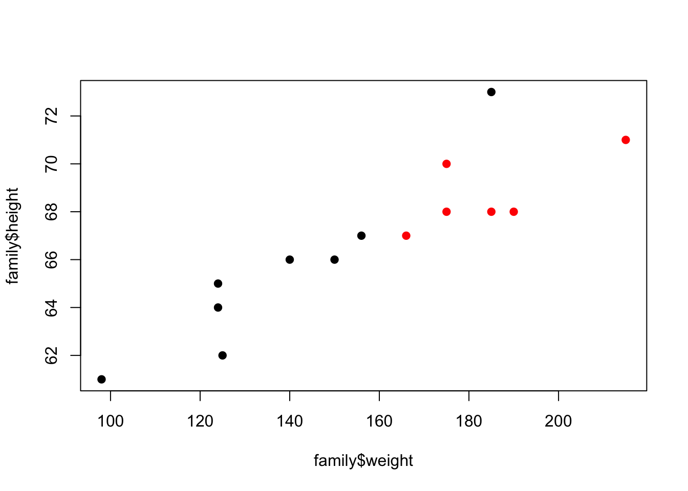
Figure 4.1: Example Scatter Plot
This scatter plot shows the heights and weights of the individuals in the artificial family that we are working with to demonstrate coding in R.
The red points correspond to over weight family members. We coerced overWt into a numeric vector with values 1 and 2 by adding 1 to each element, i.e., 1 + family$overWt. These numbers correspond to the colors black and red. The resulting plot appears in Figure 4.1
4.2 Applying Functions to Vectors in a Data Frame
Often, we want to apply a function to each variable in a data frame. For example, we may want to know each vector’s class. We have seen already that we can find this information for one vector with the $-notation, e.g.,
class(family$sex) ## [1] "factor"However, it is cumbersome to call class() 7 times, once for each of the variables, and we also need to know all of the variable names to make these 7 calls. Instead, we can ask R to apply the class() function to each of the vectors in family with
sapply(family, class)## firstName sex age height weight bmi
## "character" "factor" "integer" "integer" "integer" "numeric"
## overWt
## "logical"The sapply() function can be very useful when we work with data frames.
sapply() accepts additional arguments which can be passed on to the function that is being applied to each vector in the data frame. See the example below for an application of this concept.
Example: Quantiles of the Family Measurements
We can find the median for each of the variables in family with,
sapply(family, median)

Error in median.default(X[[2L]], ...) : need numeric data
In addition: Warning message:
In mean.default(sort(x, partial = half + 0L:1L)[half + 0L:1L]) :
  argument is not numeric or logical: returning NA
Unfortunately, since firstName and sex are character and factor vectors, respectively, the median() function returns an error indicating that it takes only numeric inputs. If we want to avoid taking the median of these two variables, we can apply the median() function to all but the first two variables by excluding them. The select() function in the dplyr package allows us to choose a subset of the variables in a data frame to work with. Below, we select columns 3, 4, …, 7 of the data frame, and pass this smaller data frame to sapply().
require(dplyr)
sapply(select(family, 3:7), median)
## age height weight bmi overWt
## 47.50000 67.00000 161.00000 24.47149 0.00000We have used subsetting to drop firstName and sex from the data frame (see Chapter ?? for more about subsetting). R applies the median() function to the remaining variables in the data frame. Also, notice that the logical vector, overWt, has been converted to numeric by the median() function.
Suppose that we want the lower quartile of these vectors, rather than the median. We can find the lower quartile for height with quantile(family$height, probs = 0.25). In addition to supplying the input family$height to the quantile() function, we also have provided the particular quantile that we want via the probs argument. In order to find the lower quantile of all the numeric vectors in family, we can use sapply(), but we need to provide the probs argument to quantile(). We can do this with
sapply(select(family,"age":"overWt"), quantile, probs = 0.25)## age.25% height.25% weight.25% bmi.25% overWt.25%
## 33.00000 65.25000 128.75000 22.71053 0.00000Notice that we subsetted the columns by name in our call to subset(). This function allows the specification of a range of variables using their names, e.g., "age":"overWt" is shorthand for c("age", "height", "weight", "bmi", "overWt"). This kind of sequence is recognized by functions in dplyr.
R offers several apply functions for working with data frames and other data structures. We only describe sapply() here. Others, such as lapply(), tapply(), and apply() are discussed in Chapter ??.
4.3 Summary: Data Frames
Data from a study or an experiment often consist of different types of measurements on a set of subjects or experimental units. For example, the World Bank provides summary statistics on countries around the world. In this case, the unit is the country and the measurements include gross domestic product, life expectancy, and literacy rate. These data are naturally organized into a table format with one row for each country and one column for each summary statistic.
The data frame is a data structure designed for the purpose of working with data that naturally organize into rows that correspond to observations/units/individuals and columns that correspond to measurements take on the observations.
Rows: Each row in a data frame corresponds to a subject in the study, unit in an experiment, etc. The various measurements on a subject are in one row of the data frame.
Columns: The columns in a data frame correspond to variables. These can be different types. For example, a health study may contain height (numeric), sex (factor), education level (orded factor), and a unique identifier (character) for all subjects.
Working with Data Frames: The data frame facilitates many kinds of statistical analyses. For example, we can easily examine the relationship between income and sex using the formula
income ~ sexin a call to theplot()function. And this same formula can be used to compare the average income levels for the two sexes via thelm()function. In both cases, the function performs a computation on the columns in a data frame. Depending on the data types, a different plot is created or a different model is fitted. For example try running the following code and comparing the results:
plot(height ~ weight, data = family)
plot(height ~ sex, data = family)

lm(height ~ weight, data = family)
lm(height ~ sex, data = family)