Chapter 2 Course Overview

“Although we often hear that data speak for themselves, their voices can be soft and sly.” – Frederick Mosteller, Stephen Fienberg, and Robert Rourke

2.1 Data-driven world

We live in a world with abundant data and these days we also have access to computing power to help us in our attempts to understand what the data are trying to tell us. In this course we want to keep the previous learning goals of Stat 20, of giving the students a solid grounding in basic statistical concepts, but now we also want to equip them with the ability to explore the data using the statistical programming language R. We hope that by the time students are finished with this course, they will feel empowered enough to download data that are interesting to them, explore these data and perhaps even draw some conclusions about what the data are saying!

2.2 Overview

We can think of our quest of understanding the data as consisting of three parts: we want to explore the data, make inferences about the data, and perhaps also predictions. We can think of statistics as inferential and descriptive. Descriptive statistics consists of numerical and graphical summaries. That is, we take snapshots of the data and visualize the data. Data visualization is very powerful and we will see some examples of both good and bad visualization, and see how bad visualization can sometimes have tragic consequences. In order to visualize the data, we will use R.

2.2.1 Generating Data

How do we collect data? Data are often collected either from observational studies or designed experiments. Of course, we can collect data just from the web, or by standing at Sproul Plaza, but it is unclear how to analyze these data. We will discuss these methods further in the chapter on sampling. At the beginning of the course we will describe what are observational studies or experiments via two well-known examples. While exploring the examples, we will introduce various statistical concepts and definitions, including randomization, types of variables. In order to understand these concepts, we will cover some basic probability at the beginning of the course, returning to probability later, when we will need it to understand statistical inference.

2.2.2 Exploring Data

We would like to get some snapshots of the data that we are going to investigate, so we will look at both numerical summaries, such as the average, percentiles, measures of spread; as well as graphical summaries including histograms and boxplots. To begin visualizing data, we will introduce the statistical programming environment R with some basic commands to get you started. We will see how to sample data, how to create histograms, and also see examples of more sophisticated visualization that we hope you will be able to reproduce in a few weeks.

2.2.3 Statistical Inference

Statistical inference is where we decipher what the data are saying. For example, we might see data that doesn’t match our expectations, but is this due to chance or is there something else going on (hypothesis tests)? Is a particular birth control pill as effective as it claims? Does a jury reflect the population? Is a company discriminating against women? Or we might use a relationship between two variables to predict values of one of them, given values of the other. This is explored in linear regression, which we will do towards the end of the semester. We will also estimate numerical quantities associated with a population, or examine such estimates - for example,the number of voters who will vote Democrat in the 2018 midterm elections. In order to do all these exciting analyses, we will need to understand some probability, since the tools we use utilize randomness. We will study random variables and their distributions and then move on to statistical inference.

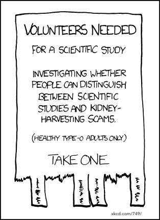
Figure 2.1: xkcd.com/749/