Contents
Introduction
Overview
Features of random forests
Remarks
How Random Forests work
The oob error estimate
Variable importance
Gini importance
Interactions
Proximities
Scaling
Prototypes
Missing values for the training set
Missing values for the test set
Mislabeled cases
Outliers
Unsupervised learning
Balancing prediction error
Detecting novelties
A case study - microarray data
Classification mode
Variable importance
Using important variables
Variable interactions
Scaling the data
Prototypes
Outliers
A case study - dna data
Missing values in the training set
Missing values in the test set
Mislabeled cases
Case Studies for unsupervised learning
Clustering microarray data
Clustering dna data
Clustering glass data
Clustering spectral data
References
Introduction
This section gives a brief overview of random forests and some comments about the features of the method.
Overview
We assume that the user knows about the construction of single classification trees. Random Forests grows many classification trees. To classify a new object from an input vector, put the input vector down each of the trees in the forest. Each tree gives a classification, and we say the tree "votes" for that class. The forest chooses the classification having the most votes (over all the trees in the forest).
Each tree is grown as follows:
- If the number of cases in the training set is N, sample N cases at random - but with replacement, from the original data. This sample will be the training set for growing the tree.
- If there are M input variables, a number m<<M is specified such that at each node, m variables are selected at random out of the M and the best split on these m is used to split the node. The value of m is held constant during the forest growing.
- Each tree is grown to the largest extent possible. There is no pruning.
In the original paper on random forests, it was shown that the forest error rate depends on two things:
- The correlation between any two trees in the forest. Increasing the correlation increases the forest error rate.
- The strength of each individual tree in the forest. A tree with a low error rate is a strong classifier. Increasing the strength of the individual trees decreases the forest error rate.
Reducing m reduces both the correlation and the strength. Increasing it increases both. Somewhere in between is an "optimal" range of m - usually quite wide. Using the oob error rate (see below) a value of m in the range can quickly be found. This is the only adjustable parameter to which random forests is somewhat sensitive.
Features of Random Forests
- It is unexcelled in accuracy among current algorithms.
- It runs efficiently on large data bases.
- It can handle thousands of input variables without variable deletion.
- It gives estimates of what variables are important in the classification.
- It generates an internal unbiased estimate of the generalization error as the forest building progresses.
- It has an effective method for estimating missing data and maintains accuracy when a large proportion of the data are missing.
- It has methods for balancing error in class population unbalanced data sets.
- Generated forests can be saved for future use on other data.
- Prototypes are computed that give information about the relation between the variables and the classification.
- It computes proximities between pairs of cases that can be used in clustering, locating outliers, or (by scaling) give interesting views of the data.
- The capabilities of the above can be extended to unlabeled data, leading to unsupervised clustering, data views and outlier detection.
- It offers an experimental method for detecting variable interactions.
Remarks
Random forests does not overfit. You can run as many trees as you want. It is fast. Running on a data set with 50,000 cases and 100 variables, it produced 100 trees in 11 minutes on a 800Mhz machine. For large data sets the major memory requirement is the storage of the data itself, and three integer arrays with the same dimensions as the data. If proximities are calculated, storage requirements grow as the number of cases times the number of trees.
How random forests work
To understand and use the various options, further information about how they are computed is useful. Most of the options depend on two data objects generated by random forests.
When the training set for the current tree is drawn by sampling with replacement, about one-third of the cases are left out of the sample. This oob (out-of-bag) data is used to get a running unbiased estimate of the classification error as trees are added to the forest. It is also used to get estimates of variable importance.
After each tree is built, all of the data are run down the tree, and proximities are computed for each pair of cases. If two cases occupy the same terminal node, their proximity is increased by one. At the end of the run, the proximities are normalized by dividing by the number of trees. Proximities are used in replacing missing data, locating outliers, and producing illuminating low-dimensional views of the data.
The out-of-bag (oob) error estimate
In random forests, there is no need for cross-validation or a separate test set to get an unbiased estimate of the test set error. It is estimated internally, during the run, as follows:
Each tree is constructed using a different bootstrap sample from the original data. About one-third of the cases are left out of the bootstrap sample and not used in the construction of the kth tree.
Put each case left out in the construction of the kth tree down the kth tree to get a classification. In this way, a test set classification is obtained for each case in about one-third of the trees. At the end of the run, take j to be the class that got most of the votes every time case n was oob. The proportion of times that j is not equal to the true class of n averaged over all cases is the oob error estimate. This has proven to be unbiased in many tests.
Variable importance
In every tree grown in the forest, put down the oob cases and count the number of votes cast for the correct class. Now randomly permute the values of variable m in the oob cases and put these cases down the tree. Subtract the number of votes for the correct class in the variable-m-permuted oob data from the number of votes for the correct class in the untouched oob data. The average of this number over all trees in the forest is the raw importance score for variable m.
If the values of this score from tree to tree are independent, then the standard error can be computed by a standard computation. The correlations of these scores between trees have been computed for a number of data sets and proved to be quite low, therefore we compute standard errors in the classical way, divide the raw score by its standard error to get a z-score, ands assign a significance level to the z-score assuming normality.
If the number of variables is very large, forests can be run once with all the variables, then run again using only the most important variables from the first run.
For each case, consider all the trees for which it is oob. Subtract the percentage of votes for the correct class in the variable-m-permuted oob data from the percentage of votes for the correct class in the untouched oob data. This is the local importance score for variable m for this case, and is used in the graphics program RAFT.
Gini importance
Every time a split of a node is made on variable m the gini impurity criterion for the two descendent nodes is less than the parent node. Adding up the gini decreases for each individual variable over all trees in the forest gives a fast variable importance that is often very consistent with the permutation importance measure.
Interactions
The operating definition of interaction used is that variables m and k interact if a split on one variable, say m, in a tree makes a split on k either systematically less possible or more possible. The implementation used is based on the gini values g(m) for each tree in the forest. These are ranked for each tree and for each two variables, the absolute difference of their ranks are averaged over all trees.
This number is also computed under the hypothesis that the two variables are independent of each other and the latter subtracted from the former. A large positive number implies that a split on one variable inhibits a split on the other and conversely. This is an experimental procedure whose conclusions need to be regarded with caution. It has been tested on only a few data sets.
Proximities
These are one of the most useful tools in random forests. The proximities originally formed a NxN matrix. After a tree is grown, put all of the data, both training and oob, down the tree. If cases k and n are in the same terminal node increase their proximity by one. At the end, normalize the proximities by dividing by the number of trees.
Users noted that with large data sets, they could not fit an NxN matrix into fast memory. A modification reduced the required memory size to NxT where T is the number of trees in the forest. To speed up the computation-intensive scaling and iterative missing value replacement, the user is given the option of retaining only the nrnn largest proximities to each case.
When a test set is present, the proximities of each case in the test set with each case in the training set can also be computed. The amount of additional computing is moderate.
Scaling
The proximities between cases n and k form a matrix {prox(n,k)}. From their definition, it is easy to show that this matrix is symmetric, positive definite and bounded above by 1, with the diagonal elements equal to 1. It follows that the values 1-prox(n,k) are squared distances in a Euclidean space of dimension not greater than the number of cases. For more background on scaling see "Multidimensional Scaling" by T.F. Cox and M.A. Cox.
Let prox(-,k) be the average of prox(n,k) over the 1st coordinate, prox(n,-) be the average of prox(n,k) over the 2nd coordinate, and prox(-,-) the average over both coordinates. Then the matrix
- cv(n,k)=.5*(prox(n,k)-prox(n,-)-prox(-,k)+prox(-,-))
is the matrix of inner products of the distances and is also positive definite symmetric. Let the eigenvalues of cv be l(j) and the eigenvectors nj(n). Then the vectors
x(n) = (Öl(1) n1(n) , Öl(2) n2(n) , ...,)
have squared distances between them equal to 1-prox(n,k). The values of Öl(j) nj(n) are referred to as the jth scaling coordinate.
In metric scaling, the idea is to approximate the vectors x(n) by the first few scaling coordinates. This is done in random forests by extracting the largest few eigenvalues of the cv matrix, and their corresponding eigenvectors . The two dimensional plot of the ith scaling coordinate vs. the jth often gives useful information about the data. The most useful is usually the graph of the 2nd vs. the 1st.
Since the eigenfunctions are the top few of an NxN matrix, the computational burden may be time consuming. We advise taking nrnn considerably smaller than the sample size to make this computation faster.
There are more accurate ways of projecting distances down into low dimensions, for instance the Roweis and Saul algorithm. But the nice performance, so far, of metric scaling has kept us from implementing more accurate projection algorithms. Another consideration is speed. Metric scaling is the fastest current algorithm for projecting down.
Generally three or four scaling coordinates are sufficient to give good pictures of the data. Plotting the second scaling coordinate versus the first usually gives the most illuminating view.
Prototypes
Prototypes are a way of getting a picture of how the variables relate to the classification. For the jth class, we find the case that has the largest number of class j cases among its k nearest neighbors, determined using the proximities. Among these k cases we find the median, 25th percentile, and 75th percentile for each variable. The medians are the prototype for class j and the quartiles give an estimate of is stability. For the second prototype, we repeat the procedure but only consider cases that are not among the original k, and so on. When we ask for prototypes to be output to the screen or saved to a file, prototypes for continuous variables are standardized by subtractng the 5th percentile and dividing by the difference between the 95th and 5th percentiles. For categorical variables, the prototype is the most frequent value. When we ask for prototypes to be output to the screen or saved to a file, all frequencies are given for categorical variables.
Missing value replacement for the training set
Random forests has two ways of replacing missing values. The first way is fast. If the mth variable is not categorical, the method computes the median of all values of this variable in class j, then it uses this value to replace all missing values of the mth variable in class j. If the mth variable is categorical, the replacement is the most frequent non-missing value in class j. These replacement values are called fills.
The second way of replacing missing values is computationally more expensive but has given better performance than the first, even with large amounts of missing data. It replaces missing values only in the training set. It begins by doing a rough and inaccurate filling in of the missing values. Then it does a forest run and computes proximities.
If x(m,n) is a missing continuous value, estimate its fill as an average over the non-missing values of the mth variables weighted by the proximities between the nth case and the non-missing value case. If it is a missing categorical variable, replace it by the most frequent non-missing value where frequency is weighted by proximity.
Now iterate-construct a forest again using these newly filled in values, find new fills and iterate again. Our experience is that 4-6 iterations are enough.
Missing value replacement for the test set
When there is a test set, there are two different methods of replacement depending on whether labels exist for the test set.
If they do, then the fills derived from the training set are used as replacements. If labels no not exist, then each case in the test set is replicated nclass times (nclass= number of classes). The first replicate of a case is assumed to be class 1 and the class one fills used to replace missing values. The 2nd replicate is assumed class 2 and the class 2 fills used on it.
This augmented test set is run down the tree. In each set of replicates, the one receiving the most votes determines the class of the original case.
Mislabeled cases
The training sets are often formed by using human judgment to assign labels. In some areas this leads to a high frequency of mislabeling. Many of the mislabeled cases can be detected using the outlier measure. An example is given in the DNA case study.
Outliers
Outliers are generally defined as cases that are removed from the main body of the data. Translate this as: outliers are cases whose proximities to all other cases in the data are generally small. A useful revision is to define outliers relative to their class. Thus, an outlier in class j is a case whose proximities to all other class j cases are small.
Define the average proximity from case n in class j to the rest of the training data class j as:
The raw outlier measure for case n is defined as
![]()
This will be large if the average proximity is small. Within each class find the median of these raw measures, and their absolute deviation from the median. Subtract the median from each raw measure, and divide by the absolute deviation to arrive at the final outlier measure.
Unsupervised learning
In unsupervised learning the data consist of a set of x -vectors of the same dimension with no class labels or response variables. There is no figure of merit to optimize, leaving the field open to ambiguous conclusions. The usual goal is to cluster the data - to see if it falls into different piles, each of which can be assigned some meaning.
The approach in random forests is to consider the original data as class 1 and to create a synthetic second class of the same size that will be labeled as class 2. The synthetic second class is created by sampling at random from the univariate distributions of the original data. Here is how a single member of class two is created - the first coordinate is sampled from the N values {x(1,n)}. The second coordinate is sampled independently from the N values {x(2,n)}, and so forth.
Thus, class two has the distribution of independent random variables, each one having the same univariate distribution as the corresponding variable in the original data. Class 2 thus destroys the dependency structure in the original data. But now, there are two classes and this artificial two-class problem can be run through random forests. This allows all of the random forests options to be applied to the original unlabeled data set.
If the oob misclassification rate in the two-class problem is, say, 40% or more, it implies that the x -variables look too much like independent variables to random forests. The dependencies do not have a large role and not much discrimination is taking place. If the misclassification rate is lower, then the dependencies are playing an important role.
Formulating it as a two class problem has a number of payoffs. Missing values can be replaced effectively. Outliers can be found. Variable importance can be measured. Scaling can be performed (in this case, if the original data had labels, the unsupervised scaling often retains the structure of the original scaling). But the most important payoff is the possibility of clustering.
Balancing prediction error
In some data sets, the prediction error between classes is highly unbalanced. Some classes have a low prediction error, others a high. This occurs usually when one class is much larger than another. Then random forests, trying to minimize overall error rate, will keep the error rate low on the large class while letting the smaller classes have a larger error rate. For instance, in drug discovery, where a given molecule is classified as active or not, it is common to have the actives outnumbered by 10 to 1, up to 100 to 1. In these situations the error rate on the interesting class (actives) will be very high.
The user can detect the imbalance by outputs the error rates for the individual classes. To illustrate 20 dimensional synthetic data is used. Class 1 occurs in one spherical Gaussian, class 2 on another. A training set of 1000 class 1's and 50 class 2's is generated, together with a test set of 5000 class 1's and 250 class 2's.
The final output of a forest of 500 trees on this data is:
500 3.7 0.0 78.4
There is a low overall test set error (3.73%) but class 2 has over 3/4 of its cases misclassified.
The error can balancing can be done by setting different weights for the classes.
The higher the weight a class is given, the more its error rate is decreased. A guide as to what weights to give is to make them inversely proportional to the class populations. So set weights to 1 on class 1, and 20 on class 2, and run again. The output is:
500 12.1 12.7 0.0
The weight of 20 on class 2 is too high. Set it to 10 and try again, getting:
500 4.3 4.2 5.2
This is pretty close to balance. If exact balance is wanted, the weight on class 2 could be jiggled around a bit more.
Note that in getting this balance, the overall error rate went up. This is the usual result - to get better balance, the overall error rate will be increased.
Detecting novelties
The outlier measure for the test set can be used to find novel cases not fitting well into any previously established classes.
The satimage data is used to illustrate. There are 4435 training cases, 2000 test cases, 36 variables and 6 classes.
In the experiment five cases were selected at equal intervals in the test set. Each of these cases was made a "novelty" by replacing each variable in the case by the value of the same variable in a randomly selected training case. The run is done using noutlier =2, nprox =1. The output of the run is graphed below:
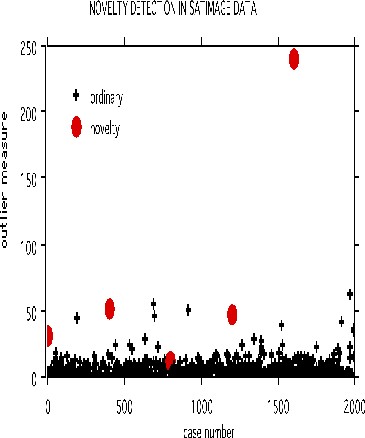
This shows that using an established training set, test sets can be run down and checked for novel cases, rather than running the training set repeatedly. The training set results can be stored so that test sets can be run through the forest without reconstructing it.
This method of checking for novelty is experimental. It may not distinguish novel cases on other data. For instance, it does not distinguish novel cases in the dna test data.
A case study-microarray data
To give an idea of the capabilities of random forests, we illustrate them on an early microarray lymphoma data set with 81 cases, 3 classes, and 4682 variables corresponding to gene expressions.
Classification mode
To do a straight classification run, use the settings:
        parameter(
c               DESCRIBE DATA
     1          mdim=4682, nsample0=81, nclass=3, maxcat=1,
     1          ntest=0, labelts=0, labeltr=1,
c
c               SET RUN PARAMETERS
     2          mtry0=150, ndsize=1, jbt=1000, look=100, lookcls=1,
     2          jclasswt=0, mdim2nd=0, mselect=0, iseed=4351,
c
c               SET IMPORTANCE OPTIONS
     3          imp=0, interact=0, impn=0, impfast=0,
c
c               SET PROXIMITY COMPUTATIONS
     4          nprox=0, nrnn=5,
c
c               SET OPTIONS BASED ON PROXIMITIES
     5          noutlier=0, nscale=0, nprot=0,
c
c               REPLACE MISSING VALUES
     6          code=-999, missfill=0,  mfixrep=0,
c
c               GRAPHICS
     7          iviz=1,
c
c               SAVING A FOREST
     8          isaverf=0, isavepar=0, isavefill=0, isaveprox=0,
c
c               RUNNING A SAVED FOREST
     9          irunrf=0, ireadpar=0, ireadfill=0, ireadprox=0)
Note: since the sample size is small, for reliability 1000 trees are grown using mtry0=150. The results are not sensitive to mtry0 over the range 50-200. Since look=100, the oob results are output every 100 trees in terms of percentage misclassified
    100 2.47
    200 2.47
    300 2.47
    400 2.47
    500 1.23
    600 1.23
    700 1.23
    800 1.23
    900 1.23
    1000 1.23
(note: an error rate of 1.23% implies 1 of the 81 cases was misclassified,)
Variable importance
The variable importances are critical. The run computing importances is done by switching imp =0 to imp =1 in the above parameter list. The output has four columns:
	gene number
	the raw importance score
	the z-score obtained by dividing the raw score by its standard error
	the significance level.
The highest 25 gene importances are listed sorted by their z-scores. To get the output on a disk file, put impout =1, and give a name to the corresponding output file. If impout is put equal to 2 the results are written to screen and you will see a display similar to that immediately below:
gene       raw     z-score  significance
number    score
  667     1.414     1.069     0.143
  689     1.259     0.961     0.168
  666     1.112     0.903     0.183
  668     1.031     0.849     0.198
  682     0.820     0.803     0.211
  878     0.649     0.736     0.231
 1080     0.514     0.729     0.233
 1104     0.514     0.718     0.237
  879     0.591     0.713     0.238
  895     0.519     0.685     0.247
 3621     0.552     0.684     0.247
 3529     0.650     0.683     0.247
 3404     0.453     0.661     0.254
  623     0.286     0.655     0.256
 3617     0.498     0.654     0.257
  650     0.505     0.650     0.258
  645     0.380     0.644     0.260
 3616     0.497     0.636     0.262
  938     0.421     0.635     0.263
  915     0.426     0.631     0.264
  669     0.484     0.626     0.266
  663     0.550     0.625     0.266
  723     0.334     0.610     0.271
  685     0.405     0.605     0.272
 3631     0.402     0.603     0.273
Using important variables
Another useful option is to do an automatic rerun using only those variables that were most important in the original run. Say we want to use only the 15 most important variables found in the first run in the second run. Then in the options change mdim2nd=0 to mdim2nd=15 , keep imp=1 and compile. Directing output to screen, you will see the same output as above for the first run plus the following output for the second run. Then the importances are output for the 15 variables used in the 2nd run.
    gene         raw       z-score    significance
   number       score
    3621 		6.235 		2.753 		0.003
    1104 		6.059 		2.709 		0.003
    3529 		5.671 		2.568 		0.005
     666 		7.837 		2.389 		0.008
    3631 		4.657 		2.363 		0.009
     667 		7.005 		2.275 		0.011
     668 		6.828 		2.255 		0.012
     689 		6.637 		2.182 		0.015
     878 		4.733 		2.169 		0.015
     682 		4.305 		1.817 		0.035
     644 		2.710 		1.563 		0.059
     879 		1.750 		1.283 		0.100
     686 		1.937 		1.261 		0.104
    1080 		0.927 		0.906 		0.183
     623 		0.564 		0.847 		0.199
Variable interactions
Another option is looking at interactions between variables. If variable m1 is correlated with variable m2 then a split on m1 will decrease the probability of a nearby split on m2 . The distance between splits on any two variables is compared with their theoretical difference if the variables were independent. The latter is subtracted from the former-a large resulting value is an indication of a repulsive interaction. To get this output, change interact =0 to interact=1 leaving imp =1 and mdim2nd =10.
The output consists of a code list: telling us the numbers of the genes corresponding to id. 1-10. The interactions are rounded to the closest integer and given in the matrix following two column list that tells which gene number is number 1 in the table, etc.
     1   2   3   4   5   6   7   8   9  10
 1   0  13   2   4   8  -7   3  -1  -7  -2
 2  13   0  11  14  11   6   3  -1   6   1
 3   2  11   0   6   7  -4   3   1   1  -2
 4   4  14   6   0  11  -2   1  -2   2  -4
 5   8  11   7  11   0  -1   3   1  -8   1
 6  -7   6  -4  -2  -1   0   7   6  -6  -1
 7   3   3   3   1   3   7   0  24  -1  -1
 8  -1  -1   1  -2   1   6  24   0  -2  -3
 9  -7   6   1   2  -8  -6  -1  -2   0  -5
10  -2   1  -2  -4   1  -1  -1  -3  -5   0
There are large interactions between gene 2 and genes 1,3,4,5 and between 7 and 8.
Scaling the data
The wish of every data analyst is to get an idea of what the data looks like. There is an excellent way to do this in random forests.
Using metric scaling the proximities can be projected down onto a low dimensional Euclidian space using "canonical coordinates". D canonical coordinates will project onto a D-dimensional space. To get 3 canonical coordinates, the options are as follows:
        parameter(
c               DESCRIBE DATA
     1          mdim=4682, nsample0=81, nclass=3, maxcat=1,
     1          ntest=0, labelts=0, labeltr=1,
c
c               SET RUN PARAMETERS
     2          mtry0=150, ndsize=1, jbt=1000, look=100, lookcls=1,
     2          jclasswt=0, mdim2nd=0, mselect=0, iseed=4351,
c
c               SET IMPORTANCE OPTIONS
     3          imp=0, interact=0, impn=0, impfast=0,
c
c               SET PROXIMITY COMPUTATIONS
     4          nprox=1, nrnn=50,
c
c               SET OPTIONS BASED ON PROXIMITIES
     5          noutlier=0, nscale=3, nprot=0,
c
c               REPLACE MISSING VALUES
     6          code=-999, missfill=0, mfixrep=0,
c
c               GRAPHICS
     7          iviz=1,
c
c               SAVING A FOREST
     8          isaverf=0, isavepar=0, isavefill=0, isaveprox=0,
c
c               RUNNING A SAVED FOREST
     9          irunrf=0, ireadpar=0, ireadfill=0, ireadprox=0)
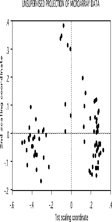
Note that imp and mdim2nd have been set back to zero and nscale set equal to 3. nrnn is set to 50 which instructs the program to compute the 50 largest proximities for each case. Set iscaleout=1. Compiling gives an output with nsample rows and these columns giving case id, true class, predicted class and 3 columns giving the values of the three scaling coordinates. Plotting the 2nd canonical coordinate vs. the first gives:
The three classes are very distinguishable. Note: if one tries to get this result by any of the present clustering algorithms, one is faced with the job of constructing a distance measure between pairs of points in 4682-dimensional space - a low payoff venture. The plot above, based on proximities, illustrates their intrinsic connection to the data.
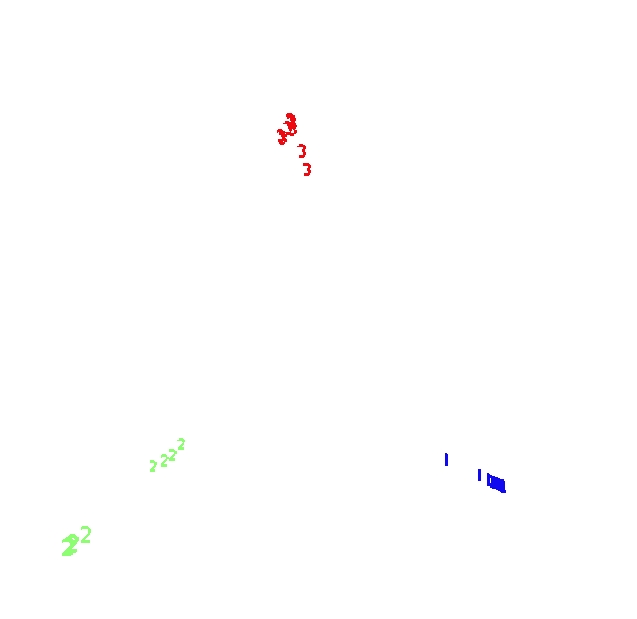
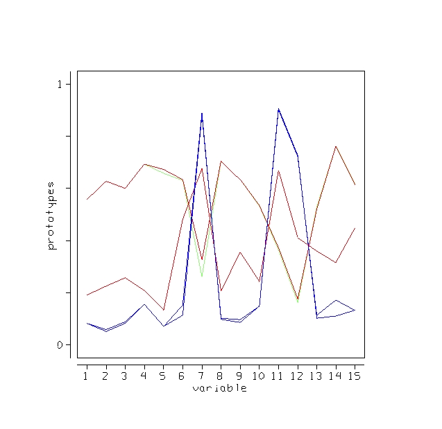
Prototypes
Two prototypes are computed for each class in the microarray data
The settings are mdim2nd=15, nprot=2, imp=1, nprox=1, nrnn=20. The values of the variables are normalized to be between 0 and 1. Here is the graph
Outliers
An outlier is a case whose proximities to all other cases are small. Using this idea, a measure of outlyingness is computed for each case in the training sample. This measure is different for the different classes. Generally, if the measure is greater than 10, the case should be carefully inspected. Other users have found a lower threshold more useful. To compute the measure, set nout =1, and all other options to zero. Here is a plot of the measure:
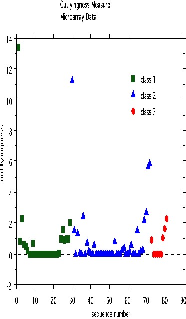
There are two possible outliers-one is the first case in class 1, the second is the first case in class 2.
A case study-dna data
There are other options in random forests that we illustrate using the dna data set. There are 60 variables, all four-valued categorical, three classes, 2000 cases in the training set and 1186 in the test set. This is a classic machine learning data set and is described more fully in the 1994 book "Machine learning, Neural and Statistical Classification" editors Michie, D., Spiegelhalter, D.J. and Taylor, C.C.
This data set is interesting as a case study because the categorical nature of the prediction variables makes many other methods, such as nearest neighbors, difficult to apply.
Missing values in the training set
To illustrate the options for missing value fill-in, runs were done on the dna data after deleting 10%, 20%, 30%, 40%, and 50% of the set data at random. Both methods missfill=1 and mfixrep=5 were used. The results are given in the graph below.
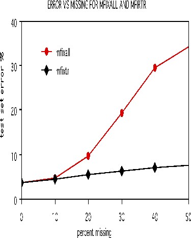
It is remarkable how effective the mfixrep process is. Similarly effective results have been obtained on other data sets. Here nrnn=5 is used. Larger values of nrnn do not give such good results.
At the end of the replacement process, it is advisable that the completed training set be downloaded by setting idataout =1.
Missing values in the test set
In v5, the only way to replace missing values in the test set is to set missfill =2 with nothing else on. Depending on whether the test set has labels or not, missfill uses different strategies. In both cases it uses the fill values obtained by the run on the training set.
We measure how good the fill of the test set is by seeing what error rate it assigns to the training set (which has no missing). If the test set is drawn from the same distribution as the training set, it gives an error rate of 3.7%. As the proportion of missing increases, using a fill drifts the distribution of the test set away from the training set and the test set error rate will increase.
We can check the accuracy of the fill for no labels by using the dna data, setting labelts=0, but then checking the error rate between the classes filled in and the true labels.
missing% labelts=1 labelts=0
  10       4.9       5.0
  20       8.1       8.4
  30      13.4      13.8
  40      21.4      22.4
  50      30.4      31.4
There is only a small loss in not having the labels to assist the fill.
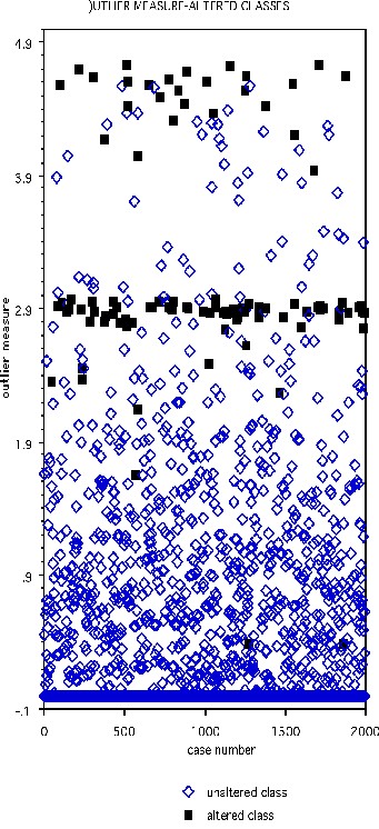
Mislabeled Cases
The DNA data base has 2000 cases in the training set, 1186 in the test set, and 60 variables, all of which are four-valued categorical variables. In the training set, one hundred cases are chosen at random and their class labels randomly switched. The outlier measure is computed and is graphed below with the black squares representing the class-switched cases
Select the threshold as 2.73. Then 90 of the 100 cases with altered classes have outlier measure exceeding this threshold. Of the 1900 unaltered cases, 62 exceed threshold.
Case studies for unsupervised learning
Clustering microarray data
We give some examples of the effectiveness of unsupervised clustering in retaining the structure of the unlabeled data. The scaling for the microarray data has this picture:
Suppose that in the 81 cases the class labels are erased. But it we want to cluster the data to see if there was any natural conglomeration. Again, with a standard approach the problem is trying to get a distance measure between 4681 variables. Random forests uses as different tack.
Set labeltr =0 . A synthetic data set is constructed that also has 81 cases and 4681 variables but has no dependence between variables. The original data set is labeled class 1, the synthetic class 2.
If there is good separation between the two classes, i.e. if the error rate is low, then we can get some information about the original data. Set nprox=1, and iscale =D-1. Then the proximities in the original data set are computed and projected down via scaling coordinates onto low dimensional space. Here is the plot of the 2nd versus the first.
The three clusters gotten using class labels are still recognizable in the unsupervised mode. The oob error between the two classes is 16.0%. If a two stage is done with mdim2nd =15, the error rate drops to 2.5% and the unsupervised clusters are tighter.
Clustering dna data
The scaling pictures of the dna data is, both supervised and unsupervised, are interesting and appear below:
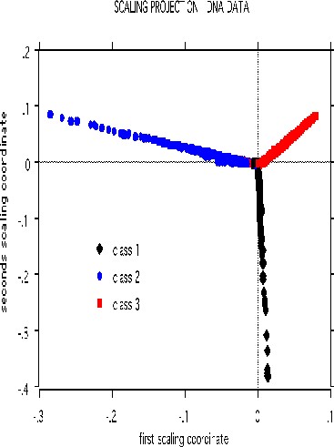
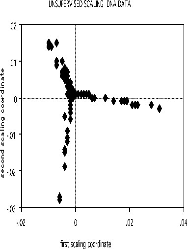
The structure of the supervised scaling is retained, although with a different rotation and axis scaling. The error between the two classes is 33%, indication lack of strong dependency.
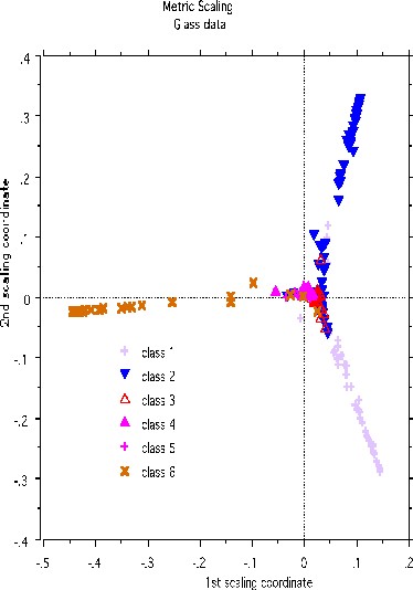
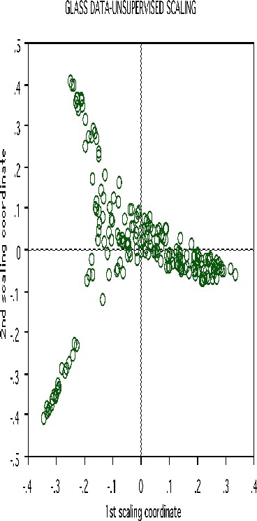
Clustering glass data
A more dramatic example of structure retention is given by using the glass data set-another classic machine learning test bed. There are 214 cases, 9 variables and 6 classes. The labeled scaling gives this picture:
Erasing the labels results in this projection:
Clustering spectral data
Another example uses data graciously supplied by Merck that consists of the first 468 spectral intensities in the spectrums of 764 compounds. The challenge presented by Merck was to find small cohesive groups of outlying cases in this data. Using forests with labeltr=0, there was excellent separation between the two classes, with an error rate of 0.5%, indicating strong dependencies in the original data.
We looked at outliers and generated this plot.
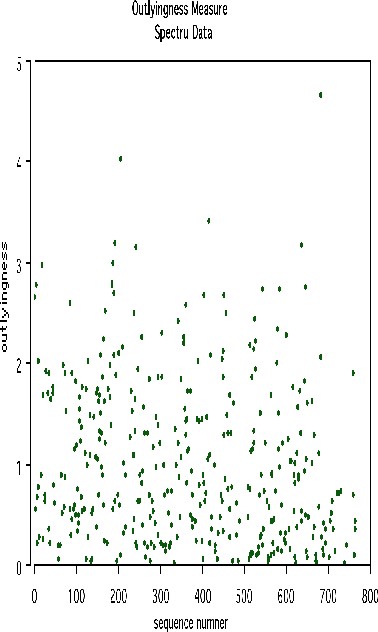
This plot gives no indication of outliers. But outliers must be fairly isolated to show up in the outlier display. To search for outlying groups scaling coordinates were computed. The plot of the 2nd vs. the 1st is below:
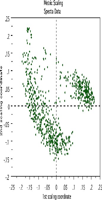
This shows, first, that the spectra fall into two main clusters. There is a possibility of a small outlying group in the upper left hand corner. To get another picture, the 3rd scaling coordinate is plotted vs. the 1st.
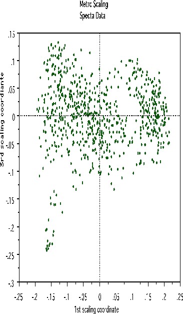
The group in question is now in the lower left hand corner and its separation from the main body of the spectra has become more apparent.
References
The theoretical underpinnings of this program are laid out in the paper "Random Forests". It's available on the same web page as this manual. It was recently published in the Machine Learning Journal.