Until now, we have been discussing the topic of probability. Roughly speaking, in probability we fully specify the distribution of some random variables, and then ask what we can say about the distribution. For example, given a complete description of the rules for generating a random walk, we might ask how long, in expectation, it will take to reach a certain threshold. This is an essentially deductive exercise: while the mathematics might be very hard, the questions we ask generally have unambiguous answers.
In statistics, we do essentially the opposite: beginning with the data — the Latin word for “given” — we work backwards to draw inferences about the data-generating distribution. This is an inductive exercise, for which the answers will inevitably be more ambiguous.
We will generally use the letter \(X\) to denote the full data set, which we assume is drawn randomly from some unknown distribution \(P\) over the sample space\(\cX\). Let \(\cP\) denote a family of candidate probability distributions, called the statistical model. We assume the analyst knows that one of the elements of \(\cP\) is the true data-generating distribution \(P\), but does not know which one. The set \(\cX\) in which \(X\) is
Example (Binomial): As a simple example, we can imagine an analyst who flips a biased coin \(n\) times, getting \(X\) heads and \(n-X\) tails. If we assume the successive flips are independent, and each has a common probability \(\theta\) of landing heads, we can write the model as
\[
X \sim \text{Binom}(n, \theta), \quad \text{ for some } \theta \in [0,1].
\]
Formally, we could say the family of distributions is \(\cP = \{\text{Binom}(n, \theta):\; \theta \in [0,1]\}\), a set of distributions indexed by the real parameter \(\theta\).
Note that in the previous example, the integer \(n\) is another important variable in the problem, but we implicitly assumed that it was “known” by the analyst, meaning that it is the same for all \(P \in \cP\). The parameter \(\theta\), by contrast, is termed “unknown” in the sense that it varies over the family \(\cP\).
Parametric vs nonparametric models
Many of the models we will consider in this class are parametric, typically meaning that they are indexed by finitely many real parameters. That is, we have \(\cP = \{P_\theta:\; \theta \in \Theta\}\), typically for some parameter space\(\Theta \subseteq \RR^d\). Then \(\theta\) is called the parameter or parameter vector.
In other models, there is no natural way to index \(\cP\) using \(d\) real numbers. We call these nonparametric models. Sometimes excited authors referred to their methods as “assumption-free,” but essentially all nonparametric models still make some assumptions about the data distribution. For example, we might assume independence between multiple observations, or shape constraints such as unimodality.
Example (Nonparameric model): Suppose we observe an i.i.d. sample of size \(n\) from a distribution \(P\) on the real line. Even if we do not want to assume anything about \(P\), the i.i.d. assumption will play an important role in the analysis. We might write this model as
\[
X_1,\ldots,X_n \simiid P, \quad \text{ for some distribution } P \text{ on } \RR.
\]
Formally, if \(X = (X_1,\ldots,X_n)\), we can write the family as \(\cP = \{P^n:\; P \text{ is a distribution on } \RR\}\), where \(P^n\) represents the \(n\)-fold product of \(P\) on \(\RR^n\).
Notation: Much of what we will learn in this course applies to parametric and nonparametric models alike, and indeed there is no crisp demarcation between parametric and nonparametric models in practice. It will often be convenient to use notation \(\cP = \{P_\theta :\; \theta \in \Theta\}\), without specifying what kind of set \(\Theta\) is; in particular there is nothing to stop \(\theta\) from being an infinite-dimensional object such as a density function. We can work in this notation without any loss of generality, since we could always take \(\theta = P\) and \(\Theta = \cP\).
Bayesian vs Frequentist inference
Thus far we have assumed the data \(X\) follows a distribution \(P_\theta\), for some unknown parameter \(\theta\) which can be any arbitrary member of the set \(\Theta\). In some contexts we will introduce an additional assumption we can call the Bayesian assumption: that \(\theta\) is itself random, drawn from some known distribution \(\Lambda\) that we call the prior.
A major advantage of this assumption is that it reduces the problem of inference about \(\theta\) to simply calculating the conditional distribution of \(\theta\) given \(X\).
The philosophical ramifications of this assumption, as well as its practical advantages and disadvantages, will be a major theme later in the course, but for now we will simply say it is an assumption we are sometimes, but not always, willing to make. From a mathematical perspective, it makes no more or less sense to assume \(\theta\) is random than it does to assume \(\theta\) is fixed and unknown.
For the remainder of this lecture, and until our unit on Bayesian inference, we will refrain from making this assumption, instead regarding \(\theta\) as taking an arbitrary fixed value in \(\Theta\).
Estimation in statistical models
Having observed \(X \sim P_\theta\), an unknown distribution in the model \(\cP = \{P_\theta:\; \theta \in \Theta\}\), we will be interested in learning something about \(\theta\). In estimation, we guess the value of some quantity of interest \(g(\theta)\), called the estimand. Our guess is called the estimate\(\delta(X)\), calculated based on the data. The method \(\delta(\cdot)\) that we use to calculate the estimate is called the estimator.
Example (Binomial, continued): Returning to our binomial example from above, we may want to estimate \(g(\theta) = \theta\), the probability of the coin landing heads. A natural estimator is \(\delta_0(X) = X/n\), the fraction of coins landing heads in any given trial. One favorable property of this estimator is that it is unbiased, meaning that \(\EE_\theta \delta_0(X) = g(\theta)\), for all \(\theta \in \Theta\).
There are many potential estimators for any given problem, so our goal will generally be to find a good estimator. To evaluate and compare estimators, we must have a way of evaluating how successful an estimator is in any given realization of the data. To this end we introduce the loss function\(L(\theta, d)\), which measures how bad it is to guess that \(g(\theta) = d\) when \(\theta\) is the true parameter value. Typically loss functions are non-negative, with \(L(\theta, d) = 0\) if and only if \(g(\theta) = d\) (no loss from a perfect guess) but this is not required.
In any given problem, we should ideally choose the loss that best measures our own true (dis)utility function, but in practice people fall back on simple defaults. One loss function that is especially popular for its mathematical convenience is the squared-error loss, defined by \(L(\theta, d) = (d-g(\theta))^2\).
Whereas the loss function measures how (un)successful an estimator is in one realization of the data, we would really like to evaluate an estimator’s performance over the whole range of possible data sets \(X\) that we might observe. This is measured by the risk function, defined as
Remark on notation: The subscript in the previous expression tells us which of our candidate probability distributions to use in evaluating the expectation. In some other fields, people may use the subscript to indicate “what randomness to integrate over,” with the implication that any random variable that does not appear in the subscript should be held fixed. In our course, it should generally be assumed that any expectation or probability is integrating over the joint distribution of the entire data set; if we want to hold something fixed we will condition on it. Recall that, for now, the parameter \(\theta\) is fixed unless otherwise specified.
The semicolon in the risk function is meant to indicate we are viewing it primarily as a function of \(\theta\). That is, we should think of and estimator \(\delta\) as having a risk function \(R(\theta)\), and the second input in \(R(\theta; \delta)\) is telling us which estimator’s risk function to evaluate at \(\theta\).
The risk for the squared-error loss is called the mean squared error (MSE):
Example (Binomial, continued): To calculate the MSE of our estimator \(\delta_0 = X/n\), note that \(\EE_\theta[X/n] = \theta\) (the estimator is unbiased). As a result, we have
One reason why we might consider estimators other than \(\delta_0\) is that, if \(n\) is small, our estimate could be quite noisy. As an extreme example, if \(n=1\) we will always estimate either \(\theta = 0\) or \(\theta = 1\), both of which would be extreme conclusions to draw after a single trial. One simple way of reducing the variance is to pretend that we flipped the coin an additional \(m\) times resulting in \(a\) heads and \(m-a\) tails. This will tend to shade our estimate toward \(a/m\), reducing the risk if \(\theta = a/m\) but possibly increasing the risk for other values of \(\theta\).
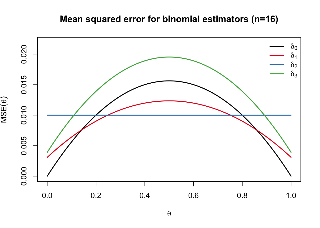
We show the risk function for several alternative estimators of this form below:
The last estimator, \(\delta_3\), is another example where we add something to \(X\) in the numerator but nothing \(n\) in the denominator.
library(RColorBrewer)n =16## risk function of estimator (X + synth.heads) / (n + synth.flips)binom.mse <-function(theta, n, synth.heads, synth.flips) { binom.var <- theta * (1- theta) * n / (n + synth.flips)^2 binom.bias <- (n * theta + synth.heads) / (n + synth.flips) - thetareturn(binom.var + binom.bias^2)}palette <-c("black",brewer.pal(4, "Set1"))curve(binom.mse(x, n, 0, 0), from=0, to=1, ylim=c(0,0.35/n), lwd=2, col=palette[1],main ="Mean squared error for binomial estimators (n=16)", ylab=expression(MSE(theta)), xlab=expression(theta))curve(binom.mse(x, n, 1, 2), add=TRUE, col=palette[2], lwd=2) curve(binom.mse(x, n, 2, 4), add=TRUE, col=palette[3], lwd=2) curve(binom.mse(x, n, 1, 0), add=TRUE, col=palette[4], lwd=2) legend("topright", col=palette, lwd=2,bty="n",legend=c(expression(delta[0]), expression(delta[1]), expression(delta[2]), expression(delta[3])))
If we look at the vertical axis, the MSE may appear to be very small, especially considering we only have 16 flips. But recall that an MSE of \(0.01\) means that we are typically missing by about \(0.1\), while estimating a parameter that is between \(0\) and \(1\).
Comparing estimators
In comparing the risk functions of these estimators, we can notice a few things. As expected, both \(\delta_1\) and \(\delta_2\) outperform \(\delta_0\) for values of \(\theta\) close to \(1/2\), but underperform for more extreme values of \(\theta\). The estimator \(\delta_3\), however, performs worse than \(\delta_0\) throughout the entire parameter space; this is because we have added bias without doing anything to reduce the variance. While it is difficult to choose between the other three estimators, we can at least rule out \(\delta_3\) on the grounds that we have no reason to ever prefer it over \(\delta_0\).
Formally, we say an estimator \(\delta\) is inadmissible if there is some other estimator \(\delta^*\) for which
\(R(\theta; \delta^*) \leq R(\theta; \delta)\) for all \(\theta\in\Theta\), and
\(R(\theta; \delta^*) < R(\theta; \delta)\) for some \(\theta\in\Theta\).
In this case we say \(\delta^*\)strictlydominates\(\delta\). An estimator is admissible if it is not inadmissible. We can see from our plot that \(\delta_3\) is inadmissible because \(\delta_0\) strictly dominates it.
Comparing the other three estimators is more difficult, however, because no one of them dominates any other. In most estimation problems, including this one, we can never hope to come up with an estimator that uniformly attains the smallest risk among all estimators. That is because, for example, we can always choose the constant estimator \(\delta(X) \equiv 1/2\) that simply ignores the data and always guesses that \(\theta = 1/2\). This estimator may perform poorly for other values of \(\theta\), but it is the only estimator that has exactly zero MSE for \(\theta = 1/2\).
If we cannot hope to minimize the risk for every value of \(\theta\) simultaneously then we must come up with some other way to resolve the inherent ambiguity in comparing all of the many estimators that we must choose among.
In our unit on estimation, we will consider two main strategies for resolving this ambiguity.
Strategy 1: Summarizing the risk function by a scalar
If we can find a way to summarize the risk function for each estimator by a single real number that we want to minimize, then we can find an estimator that is optimal in this summary sense. The two main ways to summarize the risk are to examine the average-case risk and the worst-case risk.
Average-case risk (Bayes estimation)
The first option is to minimize some (weighted) average of the risk function over the parameter space \(\Theta\) :
The average is taken with respect to some measure \(\Lambda\) of our choosing. If \(\Lambda(\Theta) < \infty\) we can assume without loss of generality that \(\Lambda\) is a probability measure, since we could always normalize it without changing the minimization problem. Then, this average is simply the estimator’s expected risk, called the Bayes risk, or equivalently the expected loss averaging over the joint distribution of \(\theta\) and \(X\). An estimator that minimizes the Bayes risk is called a Bayes estimator.
In the binomial problem above, \(\delta_1(X) = \frac{X + 1}{n + 2}\) is a Bayes estimator that minimizes the average-case risk with respect to the Lebesgue measure on \(\Theta = [0,1]\). \(\delta_2(X) = \frac{X+2}{n+4}\) is also a Bayes estimator with respect to a different prior, specifically the \(\textrm{Beta}(2,2)\) distribution. We will show this later.
Note that minimizing the average-case risk may be a natural thing to do regardless of whether we “really believe” that \(\theta \sim \Lambda\). Hence Bayes estimators are well-motivated even from a purely frequentist perspective; using them does not have to imply one has any specific position on the philosophical interpretation of probability.
If \(\Lambda(\Theta) = \infty\) then we call \(\Lambda\) an improper prior, and we can no longer interpret the corresponding Bayes risk as an expectation. But, as we will see, working with improper priors can sometimes be convenient and often leads to good estimators in practice.
Worst-case risk (Minimax estimation)
If we are reluctant to average over the parameter space, we can instead seek to minimize the worst-case risk over the entire parameter space:
This minimization problem has a game-theoretic interpretation if we imagine that, after we choose our estimator, Nature will adversarially choose the least favorable parameter value.
As we will see, minimax estimation is closely related to Bayes estimation and the minimax estimator is commonly a Bayes estimator.
The minimax perspective pushes us to choose estimators with flat risk functions, and indeed \(\delta_2(X) = \frac{X + 2}{X + 4}\) is the minimax estimator when \(n = 16\).
Strategy 2: Restricting the choice of estimators
The second main strategy for resolving ambiguity is to restrict ourselves to choose an estimator that satisfies some additional side constraint.
Unbiased estimation
One property we might want to demand of an estimator is that it be unbiased, meaning that \(\EE_\theta [\delta_0(X)] = g(\theta)\), for all \(\theta\in\Theta\). This rules out, for example, estimators that ignore the data and always guess the same value.
As we will see, once we requiring unbiasedness there will often be a clear winner among all remaining estimators under consideration, called the uniformly minimum variance unbiased (UMVU) estimator, which uniformly minimizes the risk for any convex loss function.
Of the four estimators we considered above, only \(\delta_0(X) = X/n\) is unbiased, and it is indeed the UMVU for this problem.