The OERSTED satellite is a project of the Danish Meteorological Institute (DMI). It is the first satellite experiment with global coverage of three-component measurements of Earth's "B-field" since NASA flew the MAGSAT mission in 1980. OERSTED will fly at considerably higher altitude than MAGSAT did, and will benefit from improvements in magnetometer technology and star-camera technology that should make its data extremely valuable as absolute three-component and total-field measurements, in addition to their value in conjunction with MAGSAT data in measuring temporal changes in Earth's magnetic field. Launch is planned for December, 1998; the expected duration of the data-collection phase of the mission is 14 months.
The sampling rate of the OERSTED instruments is higher than that of MAGSAT as well (25-100Hz versus about 16Hz), so high, in fact, that it is currently impractical to use the full anticipated data set to estimate properties of Earth's main magnetic field. Instead, the community prefers to have some summary measurements at a lower effective sampling rate of about 1Hz, combining observations over one-second intervals to improve the signal-to-noise ratio. An estimate of the residual uncertainty in these summary measurements is essential to making inferences about the main field from them. Two complications in reducing the sampling rate are
Simply averaging the measurements over 1s intervals was rejected, because of the possibility of nonlinear changes in the field over such intervals: if the field changes nonlinearly, the temporal average does not correspond to the value at the midpoint of the time interval.
I have implemented what I believe to be a reasonable and practical procedure for reducing the OERSTED sampling rate. It is clearly a compromise. This document reports the procedure and the results of testing it on synthetic data, data from MAGSAT, and data from ground tests of the OERSTED instrument. The algorithms are all implemented in MATLAB; this document, the algorithms, and the test data, are available over the World-Wide Web to those who wish to test them independently, to criticise them, to improve them, or to develop alternatives.
The basic procedure is to fit Chebychev polynomials to 1s intervals of data using robustly reweighted iterative least squares, and report the value of the fitted polynomial at the desired sampling point as the reduced-rate sample, with the uncertainty estimated by the bootstrap variability of the fitted values under repeatedly resampling the residuals and re-fitting:
For intervals of 100 data, fitting Chebychev polynomials of degree 4, and resampling with the bootstrap 100 times (i.e., producing 100 sets of 100 pseudo-data and fitting each set iteratively), the procedure will run in real time on an UltraSPARC (in Matlab on a 166MHz Pentium machine, it takes less than a minute). Using polynomials of degree 4 seems to work well for intervals of 100 points; degree 3 works well for intervals of 25 points. Further economies could be attained by limiting the number of iterations to, say, three.
Matlab routines implementing the approach are available. These could be translated to C or Fortran, to improve the computational efficiency.
I use a recursion relation to construct the Chebychev polynomials, which produces polynomials orthogonal with respect to the sample points to a very high degree of accuracy (10-16 or so). I normalized the polynomials to unit l2-norm by force.
The iterative least-squares fit uses the QR decomposition for stability. Because the design points are regularly spaced (except for drop-outs, which are expected to be rare), I ignore the "leverage" in computing robust weights. That is, the x-coordinate does not affect the weight assigned to a given y-residual: the weights depend on the difference (observed datum - predicted value) only.
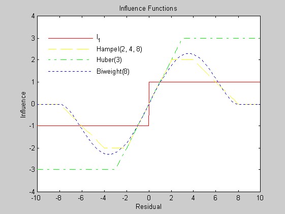
I considered four families of weight function: one corresponding to minimum l1 estimation, the Hampel weight function, the Huber minimax weight function, and Tukey's biweight function. These are implemented in l1wght.m, hampel.m, huber.m, and biwght.m.
The influence function of an estimate at the point x is essentially the change in the estimate when an infinitesmal observation is added at the point x, divided by the mass of the observation. An M-estimate is one that can be characterized as the solution of an optimization problem involving a sum of identical functions of the data. ...... For M-estimates, which include weighted least-squares, the influence function is the derivative of the weight function. The influence function gives the infinitesmal sensitivity of the solution to the addition of a new datum. data.
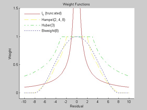
The influence functions corresponding to the biweight and to Hampel's weight redescend, so in principle, they should provide better protection against gross outliers than the l1 weight function or the Huber weight function. The figures below plot the influence functions and the corresponding weight functions. (Matlab script that generated the figures.) In practice, the l1 weight function needs to be truncated near the origin to avoid singularity. I truncated (somewhat arbitrarily) at the reciprocal of the cube-root of machine precision.
Tests comparing the performance (in a variety of senses) of some of the weight functions are described in detail below.
Minimum l1 fitting seemed not to work as well when there were gross outliers (perhaps because its influence function does not redescend), and computing the minimum l1 fit by linear programming is rather inefficient; using the weight function above and iteratively reweighted least squares, minimum l1 takes far more iterations to converge than fitting using the redescending influence functions. (I have found bugs in Matlab's linear programming routine, so I do not trust them.) I decided to restrict most of my attention to weight functions corresponding to redescending influence functions, namely, the biweight and the Hampel weight. Because the expected proportion of outliers is extremely small (less than 1%), I used a rather large parameter in the biweight (8), and corresponding parameters in the Hampel weight (2, 4, 8). If inspection of the OERSTED data once the mission is underway shows a higher fraction of outliers, the choice of parameters should be revisited.
The Hampel and Huber weights and Tukey's biweight require an estimate of the scale of the residuals, that is, something like the standard deviation of the noise. I tried several more-or-less robust approaches to estimating the scale, all based on the median absolute deviation, which is maximally robust (it has a breakdown point of 1/2):
1.483*(median absolute deviation of the deviations of the data from their median)
1.483*(median absolute deviation of the residuals from a polynomial fitted by ordinary least-squares)
A two-step procedure:
Step 1: use 1.483*(median absolute deviation of the data
from their median) to get a preliminary scale estimate;
make one weighted least-squares iteration using that
scale estimate.
Step 2: use 1.483*(median absolute deviation of the
residuals from that first weighted least-squares fit) in
all subsequent iterations.
The factor 1.483 is the ratio of the standard deviation of a normal random variable to its median absolute deviation (MAD); 1.483 times the MAD is a common robust estimate of scale. The third approach seemed to work best: the first is clearly an overestimate of the scale (because it ignores the variation of the deterministic part of the regression function), and the second approach is not as robust.
Handling missing data is straightforward; see magsTest.m for one way of doing it. Perhaps a better way is to construct the Chebychev polynomial matrix for differing numbers of points, although that would make it necessary to recompute the design matrix occasionally (the reason for using Chebychev polynomials is that they can be constructed to be orthogonal with respect to the data sampling, so that the least squares procedure is extremely stable; however, I haven't exploited the diagonality of the Gram matrix in the code, so it will handle other functional forms equally easily).
I've tested the procedure on simulated data with a variety of signal-to-noise ratios, using as the error distribution (i) a normal distribution, (ii) a uniform times a lognormal, (iii) a lognormal with random sign, (iv) a normal divided by a uniform (Tukey's "slash" distribution), which has extremely long tails, and (v) a mixture of a normal and a lognormal with random sign. I've also tried it on the OERSTED ground test data I got from Torben Risbo, and on some MAGSAT data (quiet and disturbed) I received from Michael Purucker. The MAGSAT data has a significant number of missing values, flagged as 99999. Because the geomagnetic component of the signal varies so slowly, and is expected to be essentially in the span of the fitted polynomials, I do not think it would be particularly advantageous to subtract a field model before fitting (a possibility suggested by Robert Langel).
I read some of the literature on robust filtering, but I think the nonparametric regression viewpoint is preferable to taking the observations to be a stochastic process, which is the assumption underlying the robust modifications of the Kalman filter, for example.
I'm still unsure about whether robustly fitted cubic smoothing splines with knots at a subset of the points would offer any improvement. If the degree of the fitted Chebychev polynomial is low (3 or 4), I don't think it will.
I must admit to not being completely comfortable yet with the whole idea: somehow, it's not clear to me whether one should be estimating the value at the midpoint (because then spatial aliasing would seem to be a problem), or some sort of average of the signal over each one-second interval. The answer depends in part on how people will model the processed data. I'd be grateful for any insights the reader might have.
Generalities. In tests using artificial data, the regression functions were pseudo-random Chebychev polynomials with independent, zero-mean Gaussian coefficients with equal variances. The artificial additive noise was independent, pseudo-random variables generated according to one of five distributions:
Normal: N(0,1).
Lognormal times a Uniform(-1,1): eN(0,1)×U(-1,1), with the lognormal and the uniform variates independent of each other.
Lognormal with a random sign: B×eN(0,1), where P(B=1) = P(B=-1) = ½, with B and the lognormal variate independent of each other.
Normal divided a Uniform(0,1): N(0,1)/U(0,1), with the normal and uniform independent of each other (Tukey's "slash" distribution).
Normal with signed lognormal contamination: (1-b)N(0,1)+b×BeN(0,1). In this case, it is the distribution of the noise that is the sum of the two component distributions. This is simulated by simulating a uniform(0,1) random variable U; if U<b, the noise is drawn from a lognormal with random sign as in (3). If U > b, the noise is drawn from a normal distribution. In the simulations, b was fixed at 0.02. This is perhaps the most realistic of the error distributions as a model of predominantly tame data errors with occasional gross outliers.
The noise level was calibrated crudely by multiplying the noise by the l2-norm of the sampled regression function, and dividing by a nominal "signal-to-noise ratio," which was fixed to be 5. That results in quite different "real" signal-to-noise ratios for the different noise distributions, because their variances are quite different. Even for normally distributed errors, 5 is probably a rather low value of the signal-to-noise ratio.
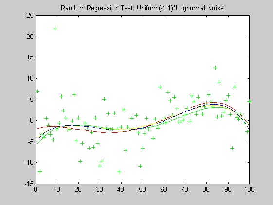
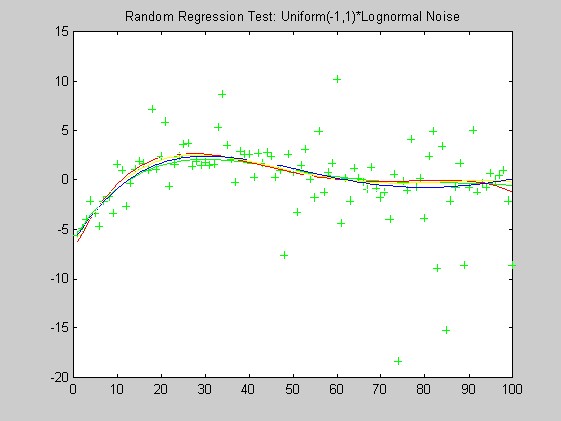
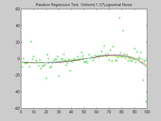
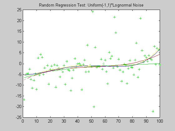
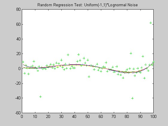
The lack of robustness of OLS compared with the other weights can be seen in these plots: OLS is generally misses the green curve by the largest distance. Based on these plots alone, I have a slight preferance for the Biweight over the Hampel weight and minimum l1.
| Additive noise in simulations | |||||||||||
| N(0,1) | eN(0,1)×U(-1,1) | BeN(0,1) | N(0,1)/U(0,1) | (1-b)N(0,1)+bBeN(0,1) | |||||||
| Biweight | Hampel | Biweight | Hampel | Biweight | Hampel | Biweight | Hampel | Biweight | Hampel | ||
| Bias | 0.14 | 0.14 | 0.04 0.02 |
-0.10 0.01 |
6.38 5.40 |
3.91 3.42 |
-0.05 | -0.41 | 0.15 0.20 |
0.17 0.26 |
|
| Relative Bias | 0.07 | 0.07 | 0.02 -0.05 |
-0.04 -0.02 |
-7.32 -16.26 |
-4.48 -10.29 |
-0.05 | -0.42 | 0.33 0.07 |
0.37 0.09 |
|
| Direct SE* | 0.76 | 1.47 | 1.18 0.41 |
0.97 0.32 |
1.18 1.00 |
0.74 0.61 |
2.15 | 3.12 | 0.92 1.00 |
1.64 1.98 |
|
| Mean ReSE** | 0.82 | 1.11 | 1.22 0.40 |
0.89 0.33 |
1.16 0.98 |
0.73 0.62 |
2.41 | 2.19 | 0.86 1.03 |
1.19 1.44 |
|
| Mean Rel. Bias of ReSE** | 0.08 | -0.25 | 0.04 -0.002 |
-0.08 0.03 |
-0.02 -0.01 |
-0.01 0.02 |
0.13 | -0.30 | -0.06 0.03 |
-0.27 -0.27 |
|
| Bias and relative bias are
estimated from 100 replications of the noise. * Standard Error estimated from 100 replications of the noise ** ReSE is the resampling estimate of the Standard Error in 100 bootstrap replications; the mean is across 100 replications of the noise. |
|||||||||||
The bias of estimates using the
biweight is generally lower than for the Hampel weight,
except for the signed lognormal error distribution. The
standard error is lower for the biweight than for the
Hampel weight for these realizations of Normal,
"slash," and lognormal-contaminated normal
errors, but higher for the uniform times the lognormal
and the signed lognormal. The relative bias of the SE
estimated by resampling is lower for the biweight for all
the error distributions except one of the realizations of
the signed lognormal. I think that is a decisive factor
in favor of the biweight: it is more important that the
error bars be "honest" than that they be short.
| true degree |
Additive noise in simulations | |||||||||||
| N(0,1) | eN(0,1)×U(-1,1) | ±eN(0,1) | N(0,1)/U(0,1) | (1-b)N(0,1)+bBeN(0,1) | ||||||||
| Biweight | Hampel | Biweight | Hampel | Biweight | Hampel | Biweight | Hampel | Biweight | Hampel | |||
| 2 | Ave. Rel. Bias | 0.02 | 0.07 | 0.11 | 0.05 | 3.40 | 2.11 | 0.48 | 0.19 | 0.12 | 0.13 | |
| Ave. |Rel. Bias| | 0.14 | 0.27 | 0.21 | 0.12 | 7.50 | 5.06 | 0.81 | 0.25 | 0.16 | 0.17 | ||
| 4* | Ave. Rel. Bias | -0.03 | -0.07 | 0.06 | 0.01 | -10.19 | -7.67 | -0.43 | -0.40 | 0.03 | 0.07 | |
| Ave. |Rel. Bias| | 0.13 | 0.31 | 0.24 | 0.08 | 11.05 | 8.22 | 1.72 | 0.83 | 0.09 | 0.13 | ||
| 6 | Ave. Rel. Bias | -0.68 | -0.80 | -0.07 | -0.06 | 6.13 | 3.49 | -0.05 | -0.41 | 0.19 | 0.20 | |
| Ave. |Rel. Bias| | 1.16 | 1.15 | 0.71 | 0.52 | 10.93 | 6.44 | 0.76 | 0.60 | 0.88 | 0.85 | ||
| * A fourth-degree (quartic) Chebychev polynomial was fitted in every case; the maximum polynomial degree of the "truth" was variously 2, 4, or 6. In the starred case, the maximum fitted degree equals the true maximum degree. | ||||||||||||
Especially for "tame" error
distributions (but also for the "slash"), the
biweight seems to be more reliable than the Hampel weight
when the true degree of the model is less than or equal
to the fitted degree.
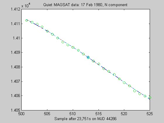
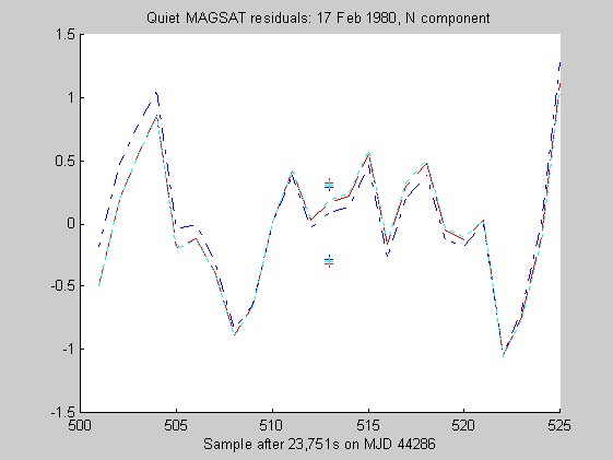
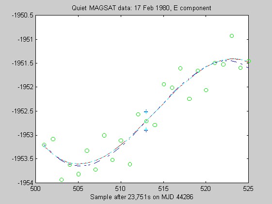
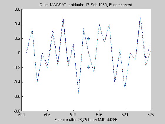
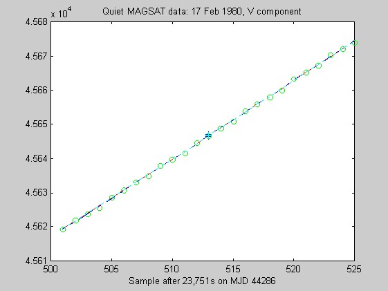
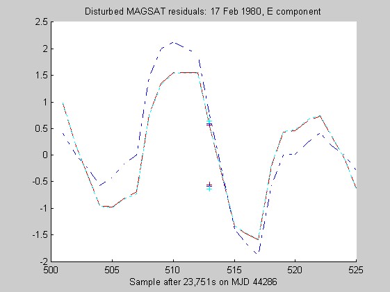
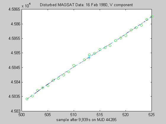
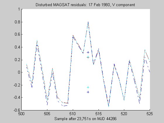
Two types of real data were available to test the algorithms: MAGSAT data (supplied by Michael Purucker), which have a different sampling rate and which were collected by a different instrument, on a satellite that flew at a different altitude from the altitude at which OERSTED will fly, and data from a ground test of the OERSTED instrument (supplied by Torben Risbo), which have a relatively small real time-varying component because the instrument was stationary relative to Earth's surface. The tests on real data are limited to visual comparisons of the fit by ordinary least squares (OLS), and iteratively reweighted least squares (IRWLS) using a variety of weight functions.
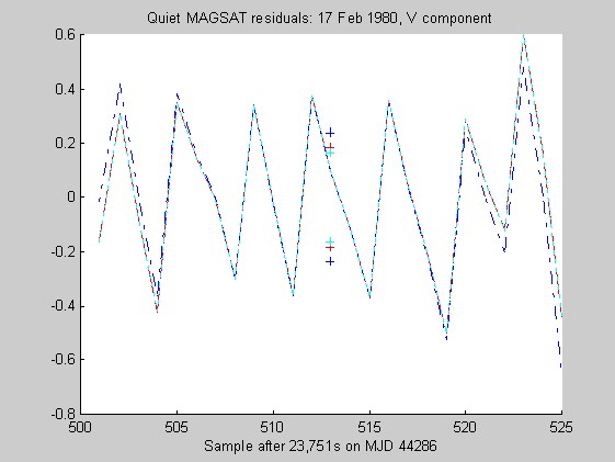
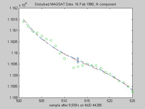
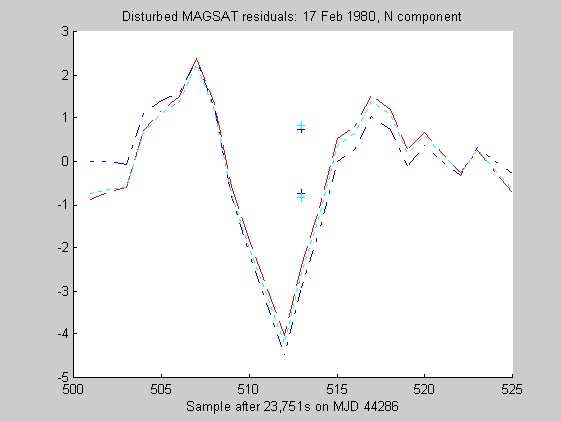
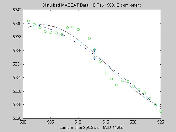
The sampling rate of the MAGSAT instrument is about 16Hz. I ran tests of the robust regression algorithms using windows of length 25 points (about 1.5s) on data collected on 16 (disturbed) and 17 (quiet) February 1980 at an average altitude of about 330km (M. Purucker, personal communication, 1996). Two sets of three pairs of plots appear below: they are for the three components of B (North, East, Vertical) at the quiet and disturbed times, showing the fits, and the residuals. In each case, cubic Chebychev polynomials were fitted. The Matlab script magsTest.m generated these plots. The plots show the MAGSAT data (green circles), the OLS fit (black), the minimum l1 fit via IRWLS (blue), the Biweight(8) fit (red), and the Hampel(2, 4, 8) fit (cyan). Approximate uncertainties of 2SE (estimated by resampling the residuals) are plotted as plusses in the same color as the corresponding curve for the reweighted (l1, Biweight and Hampel) estimates of the value at the midpoint. Each plot of fit is followed by a plot of the residuals to the fit; on the residual plots, the data would lie on a horizontal line. For reasons I do not understand, the fits using Hampel weights sometimes went awry; in extreme cases, singular matrices arose during the iterations. This happened particularly when the degree of the fitted polynomial grew. The l1 fit seemed to get confused at times, its convergence was sometimes quite slow, and I judge it inferior to the Biweight and the Hampel-weighted fits. Because of the occasional instability of the Hampel-weighted fits, the Biweight seems to be best.
Torben Risbo supplied me with ground test data from the OERSTED instrument taken at a sampling rate of 25Hz on 18 March 1996, with the instrument inside field coils, on a geomagnetically quiet day. Below are 9 plots similar to those above (using 25 samples at a time and fitting cubic Chebychev polynomials), but for the OERSTED test data. I do not know the orientation of the instrument, so I refer to the three orthogonal components of B as merely components 1-3.
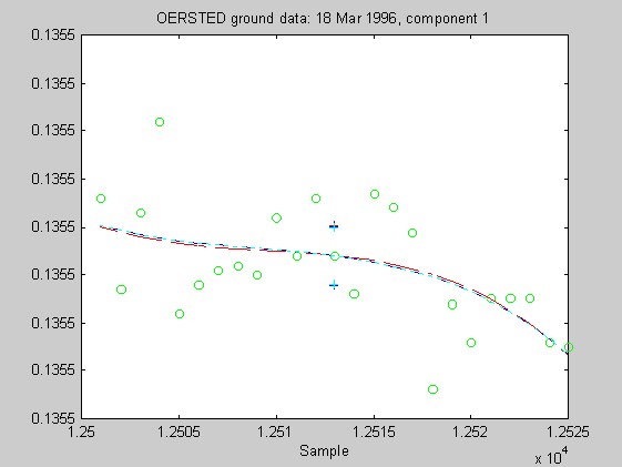
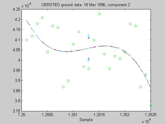
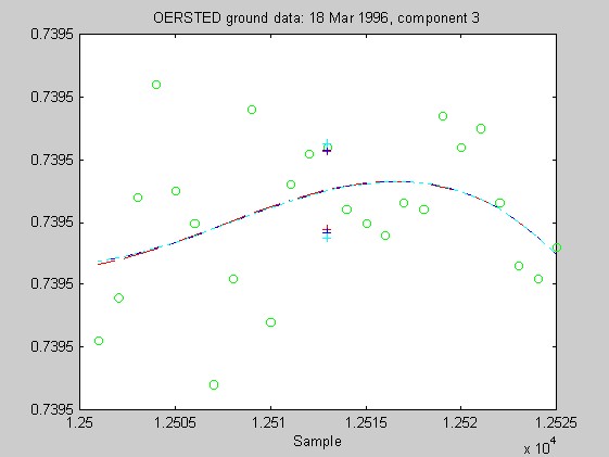
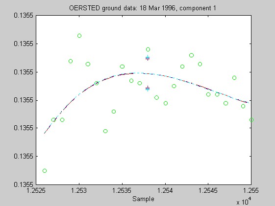
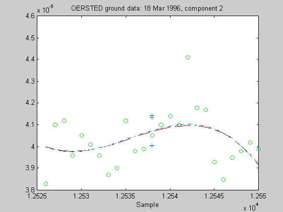
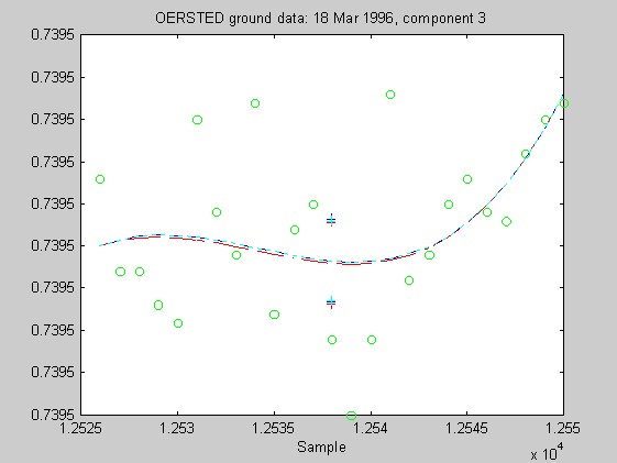
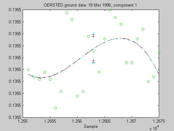
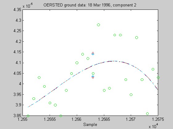
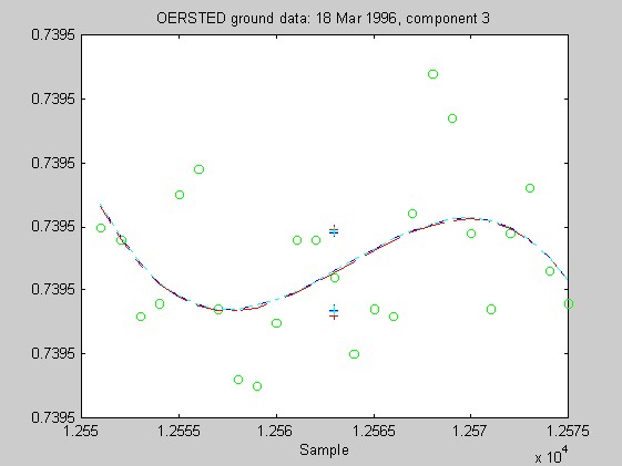
Again, the biweight appears to yield more reliable and stable regressions than both the l1 and Hampel weights. In these examples, the Hampel-weighted fits essentially follow the OLS fits. These observations, together with the facts that the biweight fit typically had a smaller relative bias in its resampling-estimated SE, and that the biweight seems less sensitive to the true degree of the underlying polynomial, make me favor the biweight for iteratively reweighted least squares fitting of the upcoming OERSTED data.
I received funding for this work from NASA through Grant NAG5-3919. I am grateful to Yoav Benjamini, Peter Bickel, Robert Langel, Torsten Neubert, Robert Parker, Fritz Primdahl, Michael Purucker, John Rice, and Torben Risbo, variously for data, helpful discussions, and suggestions.
©1997, 1998, P.B.
Stark. All rights reserved.
Last modified 13 May 1998.