Data Frames and Plotting

1 Reading Data Frames from Files and URLs

It's actually pretty rare to enter a data frame the way we've done in these examples; usually you'll be reading data from a file or possibly a URL. In these cases, the read.table function (or one of its' closely related variations described below) can be used. read.table tries to be clever about figuring out what type of data you'll be using, and automatically determines how each column of the data frame should be stored. One problem with this scheme is has to do with a special type of variable known as a factor. A factor in R is a variable that is stored as an integer, but displayed as a character string. By default, read.table will automatically turn all the character variables that it reads into factors. You can recognize factors by using either the is.factor function or by examining the objects class, using the class function. Factors are very useful for storing large data sets compactly, as well as for statistical modeling and other tasks, but when you're first working with R they'll most likely just get in the way. To avoid read.table from doing any factor conversions, pass the stringsAsFactors=TRUE argument as shown in the examples below.

By default, R expects there to be at least one space or tab between each of the data values in your input file; if you're using a different character to separate your values, you can specify it with the sep= argument. Two special versions of read.table are provided to handle two common cases: read.csv for files where the data is separated by commas, and read.delim when a tab character is used to separate values. On the other hand, if the variables in your input data occupy the same columns for every line in the file, the read.fwf can be used to turn your data into a data frame.

If the first line of your input file contains the names of the variables in your data separated with the same separator used for the rest of the data, you can pass the header=TRUE argument to read.table and its variants, and the variables (columns) of your data frame will be named accordingly. Otherwise, names like V1, V2, etc. will be used.

As an example of how to read data into a data frame, the URL http://www.stat.berkeley.edu/~spector/s133/data/world.txt contains information about literacy, gross domestic product, income and military expenditures for about 150 countries. Here are the first few lines of the file:

country,gdp,income,literacy,military
Albania,4500,4937,98.7,56500000
Algeria,5900,6799,69.8,2.48e+09
Angola,1900,2457,66.8,183580000
Argentina,11200,12468,97.2,4.3e+09
Armenia,3900,3806,99.4,1.35e+08

Since the values are separated by commas, and the variable names can be found in the first line of the file, we can read the data into a data frame as follows:

world = read.csv('http://www.stat.berkeley.edu/~spector/s133/data/world.txt',header=TRUE,stringsAsFactors=FALSE)

Now that we've created the data frame, we need to look at some ways to understand what our data is like. The class and mode of objects in R is very important, but if we query them for our data frame, they're not very interesting:

> mode(world)
[1] "list"
> class(world)
[1] "data.frame"

Note that a data frame is also a list. We'll look at lists in more detail later. In order to see the modes and classes of the individual columns, we can use the sapply function. This function will apply a function to each element of a list; for a data frame these elements represent the columns (variables), so it will do exactly what we want:

> sapply(world,mode)
    country         gdp      income    literacy    military
"character"   "numeric"   "numeric"   "numeric"   "numeric"
> sapply(world,class)
    country         gdp      income    literacy    military
"character"   "integer"   "integer"   "numeric"   "numeric"

You might want to experiment with sapply using other functions to get familiar with some strategies for dealing with data frames.

You can always view the names of the variables in a data frame by using the names function, and the size (number of observations and number of variables) using the dim function:

> names(world)
[1] "country"  "gdp"      "income"   "literacy" "military"
> dim(world)
[1] 154   5

Suppose we want to see the country for which military spending is the highest. We can still use logical subscripts just as we did with vectors, but extra care is needed to make sure we get the piece of the data frame we want. Since each country occupies one row in the data frame, we want all of the columns in that row, and we can leave the second index of the data frame blank:

>
> world[world$military == max(world$military,na.rm=TRUE),]
    country   gdp income literacy  military
141     USA 37800  39496     99.9 3.707e+11

The 141 at the beginning of the line is the row number of the observation. If you'd like to use a more informative label for the rows, look at the row.names= argument in read.table and data.frame, or use the assignment form of the row.names function if the data frame already exists.

These types of queries, where we want to find observations from a data frame that have certain properties, are so common that R provides a function called subset to make them easier and more readable. The subset function requires two arguments: the first is a data frame, and the second is the condition that you want to use to create the subset. An optional third argument called select= allows you to specify which of the variables in the data frame you're interested in. The return value from subset is a data frame, so you can use it anywhere that you'd normally use a data frame. A very attractive feature of subset is that you can refer to the columns of a data frame directly in the second or third arguments; you don't need to keep retyping the data frame's name, or surround all the variable names with quotes. So the previous query could be rewritten as:

> subset(world,military==max(military,na.rm=TRUE))
    country   gdp income literacy  military
141     USA 37800  39496     99.9 3.707e+11

One other nice feature of the select= argument is that it converts variable names to numbers before extracting the requested variables, so you can use "ranges" of variable names to specify contiguous columns in a data frame. For example, here are the names for the world data frame:

> names(world)
[1] "country"  "gdp"      "income"   "literacy" "military"

To create a data frame with just the last three variables, we could use

> subset(world,select=income:military)

If we were interested in a particular variable, it would be useful to reorder the rows of our data frame so that they were arranged in descending or ascending order of that variable. It's easy enough to sort a variable in R; using literacy as an example, we simply call the sort routine:

> sort(world$literacy)
 [1] 12.8 14.4 19.0 25.5 29.6 33.6 39.3 39.6 41.0 41.1 41.5 46.5 47.0 48.6 48.6
[16] 48.7 49.0 50.7 51.2 51.9 53.0 54.1 55.6 56.2 56.7 57.3 58.9 59.0 61.0 64.0
[31] 64.1 65.5 66.8 66.8 67.9 67.9 68.7 68.9 69.1 69.4 69.8 70.6 71.0 73.6 73.6
[46] 74.3 74.4 75.7 76.7 76.9 77.0 77.3 78.9 79.2 79.4 79.7 80.0 81.4 81.7 82.4
[61] 82.8 82.9 82.9 84.2 84.3 85.0 86.5 86.5 87.6 87.7 87.7 87.7 87.9 87.9 88.0
[76] 88.3 88.4 88.7 89.2 89.9 90.0 90.3 90.3 90.4 90.9 91.0 91.0 91.6 91.9 91.9
[91] 92.5 92.5 92.6 92.6 92.7 92.9 93.0 94.2 94.6 95.7 95.8 96.2 96.5 96.8 96.8
[106] 96.9 96.9 97.2 97.2 97.3 97.7 97.7 97.8 98.1 98.2 98.5 98.5 98.7 98.7 98.8
[121] 98.8 99.3 99.3 99.4 99.4 99.5 99.5 99.6 99.6 99.6 99.7 99.7 99.7 99.8 99.9
[136] 99.9 99.9 99.9 99.9 99.9 99.9 99.9 99.9 99.9 99.9 99.9 99.9 99.9 99.9 99.9
[151] 99.9 99.9 99.9 99.9

To reorder the rows of a data frame to correspond to the sorted order of one of the variables in the data frame, the order function can be used. This function returns a set of indices which are in the proper order to rearrange the data frame appropriately:

> sworld = world[order(world$literacy),]
> head(sworld)
         country  gdp income literacy  military
22  Burkina Faso 1100   1258     12.8  64200000
103        Niger  800    865     14.4  33300000
89          Mali  900   1024     19.0  22400000
29          Chad 1200   1555     25.5 101300000
121 Sierra Leone  500    842     29.6  13200000
14         Benin 1100   1094     33.6  96500000

To sort by descending values of a variable, pass the decreasing=TRUE argument to sort or order.

When you're first working with a data frame, it can be helpful to get some preliminary information about the variables. One easy way to do this is to pass the data frame to the summary function, which understands what a data frame is, and will give separate summaries for each of the variables:

> summary(world)
   country               gdp            income         literacy
 Length:154         Min.   :  500   Min.   :  569   Min.   :12.80
 Class :character   1st Qu.: 1825   1st Qu.: 2176   1st Qu.:69.17
 Mode  :character   Median : 4900   Median : 5930   Median :88.55
                    Mean   : 9031   Mean   :10319   Mean   :81.05
                    3rd Qu.:11700   3rd Qu.:15066   3rd Qu.:98.42
                    Max.   :55100   Max.   :63609   Max.   :99.90
                                    NA's   :    1
    military
 Min.   :6.500e+06
 1st Qu.:5.655e+07
 Median :2.436e+08
 Mean   :5.645e+09
 3rd Qu.:1.754e+09
 Max.   :3.707e+11

Another useful way to view the properties of a variable is with the stem function, which produces a text-base stem-and-leaf diagram. Each observation for the variable is represented by a number in the diagram showing that observation's value:

> stem(world$gdp)

  The decimal point is 4 digit(s) to the right of the |

  0 | 11111111111111111111111111112222222222222222222223333333333344444444
  0 | 55555555555666666666677777778889999
  1 | 000111111223334
  1 | 66788889
  2 | 0022234
  2 | 7778888999
  3 | 00013
  3 | 88
  4 |
  4 |
  5 |
  5 | 5

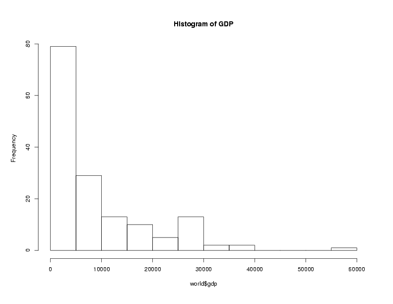
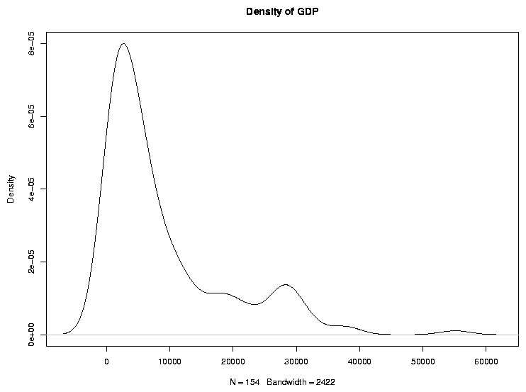
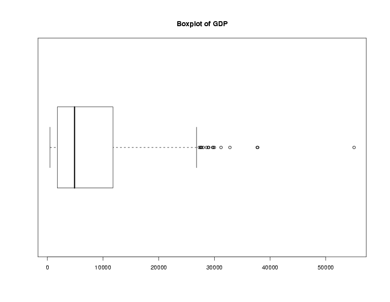
Graphical techniques are often useful when exploring a data frame. While we'll look at graphics in more detail later, the functions boxplot, hist, and plot combined with the density function are often good choices. Here are examples:

> boxplot(world$gdp,main='Boxplot of GDP')
> hist(world$gdp,main='Histogram of GDP')
> plot(density(world$gdp),main='Density of GDP')

Suppose we want to add some additional information to our data frame, for example the continents in which the countries can be found. Very often we have information from different sources and it's very important to combine it correctly. The URL http://www.stat.berkeley.edu/s133/data/conts.txt contains the information about the continents. Here are the first few lines of that file:

country,cont
Afghanistan,AS
Albania,EU
Algeria,AF
American Samoa,OC
Andorra,EU

In R, the merge function allows you to combine two data frames based on the value of a variable that's common to both of them. The new data frame will have all of the variables from both of the original data frames. First, we'll read in the continent values into a data frame called conts:

conts = read.csv('http://www.stat.berkeley.edu/~spector/s133/data/conts.txt',na.string='.',stringsAsFactors=FALSE)

To merge two data frames, we simply need to tell the merge function which variable(s) the two data frames have in common, in this case country:

world1 = merge(world,conts,by='country')

Notice that we pass the name of the variable that we want to merge by, not the actual value of the variable itself. The first few records of the merged data set look like this:

> head(world1)
    country   gdp income literacy   military cont
1   Albania  4500   4937     98.7 5.6500e+07   EU
2   Algeria  5900   6799     69.8 2.4800e+09   AF
3    Angola  1900   2457     66.8 1.8358e+08   AF
4 Argentina 11200  12468     97.2 4.3000e+09   SA
5   Armenia  3900   3806     99.4 1.3500e+08   AS
6 Australia 28900  29893     99.9 1.6650e+10   OC

We've already seen how to count specific conditions, like how many countries in our data frame are in Europe:

> sum(world1$cont == 'EU')
[1] 34

It would be tedious to have to repeat this for each of the continents. Instead, we can use the table function:

> table(world1$cont)

AF AS EU NA OC SA
47 41 34 15  4 12

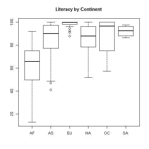
We can now examine the variables taking into account the continent that they're in. For example, suppose we wanted to view the literacy rates of countries in the different continents. We can produce side-by-side boxplots like this:

> boxplot(split(world1$literacy,world1$cont))

Now let's concentrate on plots involving two variables. It may be surprising, but R is smart enough to know how to "plot" a dataframe. It actually calls the pairs function, which will produce what's called a scatterplot matrix. This is a display with many little graphs showing the relationships between each pair of variables in the data frame. Before we can call plot, we need to remove the character variables (country and cont) from the data using negative subscripts:

> plot(world1[,-c(1,6)])

The resulting plot looks like this:

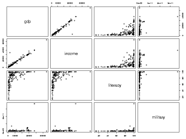As we'd expect, gdp (Gross Domestic Product) and income seem to have a very consistent relationship. The relation between literacy and income appears to be interesting, so we'll examine it in more detail, by making a separate plot for it:

> with(world,plot(literacy,income))

The first variable we pass to plot (literacy in this example) will be used for the x-axis, and the second (income) will be used on the y-axis. The plot looks like this:

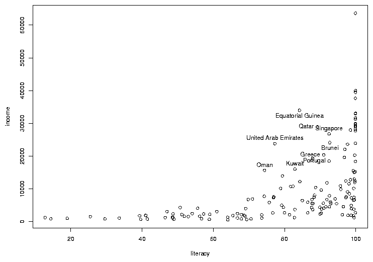
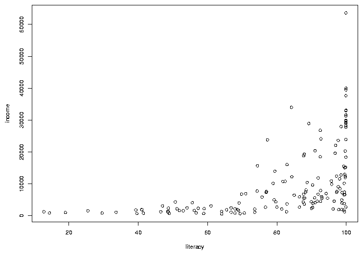In many cases, the most interesting points on a graph are the ones that don't follow the usual relationships. In this case, there are a few points where the income is a bit higher than we'd expect based on the other countries, considering the rate of literacy. To see which countries they represent, we can use the identify function. You call identify with the same arguments as you passed to plot; then when you click on a point on the graph with the left mouse button, its row number will be printed on the graph. It's usually helpful to have more than just the row number, so identify is usually called with a labels= argument. In this case, the obvious choice is the country name. The way to stop identifying points depends on your operating system; on Windows, right click on the plot and choose "Stop"; on Unix/Linux click on the plot window with the middle button. Here's the previous graph after some of the outlier points are identified:

File translated from T_EX by T_TH, version 3.67.
On 1 Feb 2010, 10:11.