Graphical User Interfaces
1 Appearance of Widgets
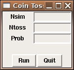
The previous example was a very minimalistic approach, with no
concern with the actual appearance of the final product. One simple
way to improve the appearance is to add a little space around the
widgets when we pack them. The tkpack function accepts two
arguments, padx= and pady= to control the amount of
space around the widgets when they are packed. Each of these arguments
takes a scalar or a vector of length 2. When a scalar is given, that much
space (in pixels) is added on either side of the widget in the specified
dimension. When a list is given the first number is the amount of space
to the left (padx) or the top (pady), and the second
number is the amount of space to the right (padx) or the bottom
(pady). Like most aspects of GUI design, experimentation is
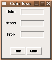
often necessary to find the best solution. The following code produces
a version of the coin power GUI with additional padding:
base = tktoplevel()
tkwm.title(base,'Coin Toss')

nfrm = tkframe(base)

nsim_ = tclVar('')
ntoss_ = tclVar('')
prob_ = tclVar('')

f1 = tkframe(nfrm)
tkpack(tklabel(f1,text='Nsim',width=8),side='left',pady=c(5,10))
tkpack(tkentry(f1,width=10,textvariable=nsim_),side='left',padx=c(0,20),pady=c(5,10))

f2 = tkframe(nfrm)
tkpack(tklabel(f2,text='Ntoss',width=8),side='left',pady=c(5,10))
tkpack(tkentry(f2,width=10,textvariable=ntoss_),side='left',padx=c(0,20),pady=c(5,10))

f3 = tkframe(nfrm)
tkpack(tklabel(f3,text='Prob',width=8),side='left',pady=c(5,10))
tkpack(tkentry(f3,width=10,textvariable=prob_),side='left',padx=c(0,20),pady=c(5,10))

tkpack(f1,side='top')
tkpack(f2,side='top')
tkpack(f3,side='top')

tkpack(nfrm)

ans = tklabel(base,text=' ')
tkpack(ans,side='top')

bfrm = tkframe(base)
tkpack(tkbutton(bfrm,text='Run',command=tst),side='left')
tkpack(tkbutton(bfrm,text='Quit',command=destroy),side='right')

tkpack(bfrm,side='bottom',pady=c(0,10))
Here are side-by-side pictures showing the difference between the two
versions:
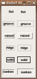
Another way to modify a GUI's appearance is through three-dimensional
effects. These are controlled by an argument called relief=,
which can take values of "flat", "groove", "raised",
"ridge", ßolid", or ßunken".
The following code produces a (non-functioning) GUI showing the different
relief styles applied to labels and buttons:
require(tcltk)
types = c('flat','groove','raised','ridge','solid','sunken')

base = tktoplevel()
tkwm.title(base,'Relief Styles')

frms = list()

mkframe = function(type){
    fr = tkframe(base)
    tkpack(tklabel(fr,text=type,relief=type),side='left',padx=5)
    tkpack(tkbutton(fr,text=type,relief=type),side='left',padx=5)
    tkpack(fr,side='top',pady=10)
    fr
}

sapply(types,mkframe)
Here's a picture of how it looks:
2 Fonts and Colors
Several arguments can be used to modify color. The background=
argument controls the overall color, while the foreground= argument
controls the color of text appearing in the widget. (Remember that things
like this can be changed while the GUI is running using the tkconfigure
command. Each of these arguments accepts colors spelled out (like
"lightblue", "red", or "green") as well as
web-style hexadecimal values (like "#add8e6", "#ff0000" or
"#00ff00").
To change from the default font (bold Helvetica), you must first create
a Tk font, using the tkfont.create function. This function takes
a number of arguments, but only the font family is required.
The available font families will vary from platform to platform; the
as.character(tkfont.families()) command will display a list of the available
fonts. Some of the other possible arguments to tkfont.create
include:
- size=, the size of the font in points.
-
weight=, either "normal" or "bold"
-
slant=, either "roman" or ïtalic"
-
underline=, either TRUE or FALSE
-
overstrike=, either TRUE or FALSE
As mentioned earlier, colors can be specified as either names or web-style
hexadecimal values. Generally, the argument to change the color of a
widget is background=; the argument to change the color of any
text appearing in the widget is foreground=. If these choices don't
do what you expect, you may need to check the widget-specific documentation.
Here's a simple program that chooses some randomly selected colors and fonts,
and displays them as labels.
require(tcltk)

allfonts = as.character(tkfont.families())
somefonts = sample(allfonts,9)

somecolors = c('red','blue','green','yellow','lightblue','tan',
'darkred','lightgreen','white')

txt = 'ABCDEFGHIJKLMNOPQRSTUVWXYZabcdefghijklmnopqrstuvwxyz'

base = tktoplevel()
tkwm.title(base,'Fonts')
mkfonts = function(font,color){
      thefont = tkfont.create(family=font,size=14)
      tkpack(tklabel(base,text=paste(font,':',txt),
                    font=thefont,background=color),
                    side='top')
}

mapply(mkfonts,somefonts,somecolors)
Here's how it looks:
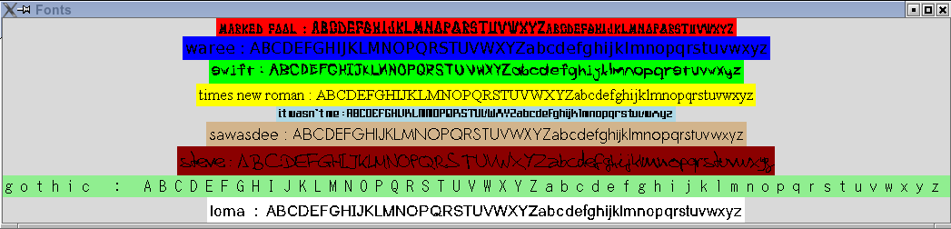 Note that only the specific widget for which background= was set
changes - if you want to change the background for the entire GUI, you'll
probably have to pass the background= argument to every widget you
use.
Note that only the specific widget for which background= was set
changes - if you want to change the background for the entire GUI, you'll
probably have to pass the background= argument to every widget you
use.
3 Plotting
When developing a TK-based GUI for plotting, there are two possibilities available.
The first, which is the only choice if you need to interact with the graph using
locator or identify, is to create a GUI with the controls for the
plot, and to let R open a normal plotting window. The second option utilizes the
tkrplot library, available from CRAN, to create a label widget with an image
of the plot; this label can be placed anywhere that any other widget can be placed.
To illustrate the use of a GUI with plotting, consider
the problem of mixtures of normal distributions. Many times a sample will
actually contain
two separate distributions, even though it will be treated as a single distribution.
Obviously data like this will create problems when we try to analyze it, so it's
important to be able to recognize such data, using, say a density plot. To get
an idea of how the density of mixtures of distributions would look, we can create
a GUI using a scale or slider widget that will allow us to control the fraction
of each of two distributions that will be combined. Many times the first step
in making a GUI is writing the function that the GUI will eventually call to
actually do the work. This helps to identify the parameters that need to be
supplied to the function so that the GUI can be designed in such a way to get all
the necessary information. For this case, we'll want to specify the mean and
standard deviation of the first distribution, the mean and standard deviation of
the second distribution, and the fraction of the second distribution to use. (The
fraction for the first distribution will just be 1 minus the fraction for the
second distribution.) Here's such a function:
genplot = function(m1,s1,m2,s2,frac,n=100){
     dat = c(rnorm((1-frac)*n,m1,s1),rnorm(frac*n,m2,s2))
     plot(density(dat),type='l',main='Density of Mixtures')
}
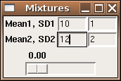
Now we can create the interface. We'll make three frames: the first will accept
the mean and standard deviation for the first distribution, the second will have
the mean and standard deviation for the second distribution, and the third will
have the slider to determine the fraction of each distribution to use. Recall that
we need to create tcl variables, and then convert them into R variables
before we can call our function, so I'll use an intermediate function which will
do the translations and then call genplot as a callback. Although there
is a fair amount of code, most of it is very similar.
require(tcltk)

doplot = function(...){
   m1 = as.numeric(tclvalue(mean1))
   m2 = as.numeric(tclvalue(mean2))
   s1 = as.numeric(tclvalue(sd1))
   s2 = as.numeric(tclvalue(sd2))
   fr = as.numeric(tclvalue(frac))
   genplot(m1,s1,m2,s2,fr,n=100)
}

base = tktoplevel()
tkwm.title(base,'Mixtures')
mainfrm = tkframe(base)

mean1 = tclVar(10)
mean2 = tclVar(10)
sd1   = tclVar(1)
sd2   = tclVar(1)
frac  = tclVar(.5)

m1 = tkframe(mainfrm)
tkpack(tklabel(m1,text='Mean1, SD1',width=10),side='left')
tkpack(tkentry(m1,width=5,textvariable=mean1),side='left')
tkpack(tkentry(m1,width=5,textvariable=sd1),side='left')
tkpack(m1,side='top')

m2 = tkframe(mainfrm)
tkpack(tklabel(m2,text='Mean2, SD2',width=10),side='left')
tkpack(tkentry(m2,width=5,textvariable=mean2),side='left')
tkpack(tkentry(m2,width=5,textvariable=sd2),side='left')
tkpack(m2,side='top')

m3 = tkframe(mainfrm)
tkpack(tkscale(m3,command=doplot,from=0,to=1,showvalue=TRUE,
               variable=frac,resolution=.01,orient='horiz'))
tkpack(m3,side='top')

tkpack(mainfrm)
Here's how the interface looks:
 To produce the same sort of GUI, but with the plot in the same frame as the
slider, we can use the tkrplot library. To place the plot in the
same frame as the slider, we must first create a tkrplot widget, using
the tkrplot function. After loading the tkrplot library,
we call this function with two arguments; the frame in which the plot is to
be displayed, and a callback function (using ... as the only argument)
that will draw the desired plot. In this example, we can use the same function
(doplot) as in the standalone version:
To produce the same sort of GUI, but with the plot in the same frame as the
slider, we can use the tkrplot library. To place the plot in the
same frame as the slider, we must first create a tkrplot widget, using
the tkrplot function. After loading the tkrplot library,
we call this function with two arguments; the frame in which the plot is to
be displayed, and a callback function (using ... as the only argument)
that will draw the desired plot. In this example, we can use the same function
(doplot) as in the standalone version:
img = tkrplot(mainfrm,doplot)
Since the tkrplot widget works by displaying an image of the
plot, the only way to change the plot is to change this image, which is exactly
what the tkrreplot function does. The only argument to tkrreplot
is the tkrplot widget that will need to be redrawn. Thus, the slider
can be constructed with the following statements:
scalefunc = function(...)tkrreplot(img)
s = tkscale(mainfrm,command=scalefunc,from=0,to=1,showvalue=TRUE,
               variable='frac',resolution=.01,orient='horiz')
By packing the tkrplot object first, followed by the frames for the mean
and standard deviations, and packing the slider widget last, we can produce the
GUI shown below:
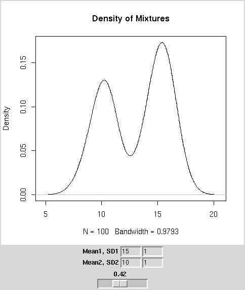 The complete code for this GUI is as follows:
require(tcltk)
require(tkrplot)

genplot = function(m1,s1,m2,s2,frac,n=100){
     dat = c(rnorm((1-frac)*n,m1,s1),rnorm(frac*n,m2,s2))
          plot(density(dat),type='l',main='Density of Mixtures')
	  }

doplot = function(...){
   m1 = as.numeric(tclvalue(mean1))
   m2 = as.numeric(tclvalue(mean2))
   s1 = as.numeric(tclvalue(sd1))
   s2 = as.numeric(tclvalue(sd2))
   fr = as.numeric(tclvalue(frac))
   genplot(m1,s1,m2,s2,fr,n=100)
}


base = tktoplevel()
tkwm.title(base,'Mixtures')
mainfrm = tkframe(base)

mean1 = tclVar(10)
mean2 = tclVar(10)
sd1   = tclVar(1)
sd2   = tclVar(1)
frac  = tclVar(.5)

img = tkrplot(mainfrm,doplot)
scalefunc = function(...)tkrreplot(img)
s = tkscale(mainfrm,command=scalefunc,from=0,to=1,showvalue=TRUE,
               variable=frac,resolution=.01,orient='horiz')
tkpack(img)

m1 = tkframe(mainfrm)
tkpack(tklabel(m1,text='Mean1, SD1',width=10),side='left')
tkpack(tkentry(m1,width=5,textvariable=mean1),side='left')
tkpack(tkentry(m1,width=5,textvariable=sd1),side='left')
tkpack(m1,side='top')
m2 = tkframe(mainfrm)
tkpack(tklabel(m2,text='Mean2, SD2',width=10),side='left')
tkpack(tkentry(m2,width=5,textvariable=mean2),side='left')
tkpack(tkentry(m2,width=5,textvariable=sd2),side='left')
tkpack(m2,side='top')

tkpack(s)

tkpack(mainfrm)
4 Binding
For those widgets that naturally have an action or variable associated
with them, the Tk interface provides arguments like textvariable=,
or command= to make it easy to get these widgets working as they
should. But we're not limited to associating actions with only those
widgets that provide such arguments. By using the tkbind command,
we can associate a function (similar to those accepted by functions
that use a command= argument) to any of a large number of possible
events. To indicate an event, a character string with the event's name
surrounded by angle brackets is used. The following table shows some of
the actions that can have commands associated with them. In the table,
a lower case x is used to represent any key on the keyboard.
| <Return> | <FocusIn> |
| <Key-x> | <FocusOut> |
| <Alt-x> | <Button-1>, <Button-2>, etc. |
| <Control-x> | <ButtonRelease-1>, <ButtonRelease-2>, etc. |
| <Destroy> | <Double-Button-1>, <Double-Button-2> , etc. |
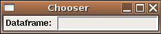
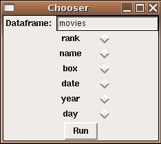
As an example, suppose we wish to create a GUI that will allow the user to
type in the name of a data frame, and when the user hits return in the
entry field, a set of radio buttons, one for each variable in the data
frame, will open up below the entry field. Finally, a button will allow
for the creation of a histogram from the selected variable.
require(tcltk)

makehist = function(...){
   df = get(tclvalue(dfname))
   thevar = tclvalue(varname)
   var = as.numeric(df[[thevar]])
   hist(var,main=paste("Histogram of",thevar),xlab=thevar)
}

showb = function(...){
    df = get(tclvalue(dfname))
    vars = names(df)
    frms = list()
    k = 1

    mkframe = function(var){
        fr = tkframe(base)
        tkpack(tklabel(fr,width=15,text=var),side='left')
        tkpack(tkradiobutton(fr,variable=varname,value=var),side='left')
        tkpack(fr,side='top')
        fr
    }

    frms = sapply(vars,mkframe)

    tkpack(tkbutton(base,text='Run',command=makehist),side='top')
}

base = tktoplevel()
tkwm.title(base,'Chooser')

dfname = tclVar()
varname = tclVar()

efrm = tkframe(base)

tkpack(tklabel(efrm,text='Dataframe: '),side='left')
dfentry = tkentry(efrm,textvariable=dfname,width=20)
tkbind(dfentry,'<Return>',showb)
tkpack(dfentry,side='left')
tkpack(efrm)
Here's a picture of the widget in both the "closed" and "open" views:
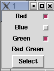
5 Checkbuttons
When we created radiobuttons, it was fairly simple, because we only needed
to create one tcl variable, which would contain the value
of the single chosen radiobutton. With checkbuttons, the user can choose
as many selections as they want, so each button must have a separate
tcl variable associated with it. While it's possible to do this
by hand for each choice provided, the following example shows how to use
the sapply function to do this in a more general way. Notice that
special care must be taken when creating a list of tcl variables to
insure that they are properly stored. In this simple example, we
print the choices, by using sapply to convert the list of tcl
variables to R variables. Remember that all the toplevel variables that you
create in an R GUI are available in the console while the GUI is running, so
you examine them in order to see how their information is stored.
require(tcltk)
tt <- tktoplevel()
choices = c('Red','Blue','Green')
bvars = lapply(choices,function(i)tclVar('0'))
# or bvars = rep(list(tclVar('0')),length(bvars))
names(bvars) = choices
mkframe = function(x){
   nn = tkframe(tt)
   tkpack(tklabel(nn,text=x,width=10),side='left')
   tkpack(tkcheckbutton(nn,variable=bvars[[x]]),side='right')
   tkpack(nn,side='top')
}

sapply(choices,mkframe)

showans = function(...){
   res = sapply(bvars,tclvalue)
   res = names(res)[which(res == '1')]
   tkconfigure(result,text = paste(res,collapse=' '))
}

result = tklabel(tt,text='')
tkpack(result,side='top')

bfrm = tkframe(tt)
tkpack(tkbutton(bfrm,command=showans,text='Select'),side='top')
tkpack(bfrm,side='top')
The figure below shows what the GUI looks like after two choices
have been made, and the button is pressed.
6 Opening Files and Displaying Text
While it would be very simple (and not necessarily a bad idea) to use an
entry field to specify a file name, the Tk toolkit provides a file browser
which will return the name of a file which a user has chosen, and will usually
be a better choice if you need to open a file.
Another issue that arises has to do with displaying output. If the output is
a plot, it's simple to just open a graph window; if the output is text, you
can just print it in the normal way, and it will display in the same place
as you typed the R command to display the GUI. While this is useful while
debugging your program, if there are printed results they should usually be
displayed in a separate window. For this purpose, Tk provides the
tktext object. To display output in this way, we can use the
capture.output function, which takes the output of any R command
and, instead of displaying it to the screen, stores the output in a
vector of character values.
Alternatively,
the output could be written to a file,
then read back into a character vector.
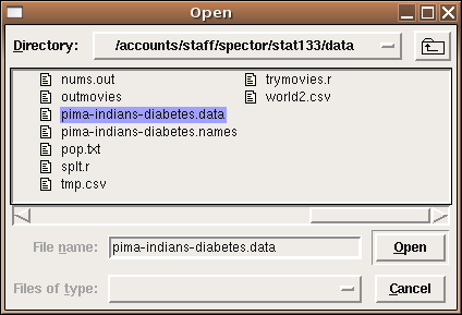
The following example program invokes tkgetOpenFile to get the name of a file
to be opened; it then opens the file, reads it as a CSV file and displays the
results in a text window with scrollbars. The wrap='none' argument
tells the text window not to wrap the lines; this is appropriate when you have
a scrollbar in the x-dimension. Finally, to give an idea of how the text
window can be modified, a button is added to change the text window's display
from the listing of the data frame to a data frame summary.
require(tcltk)

summ = function(...){
   thestring = capture.output(summary(myobj))
   thestring = paste(thestring,collapse='\n')
   tkdelete(txt,'@0,0','end')
   tkinsert(txt,'@0,0',thestring)
}

fileName<-tclvalue(tkgetOpenFile())

myobj = read.csv(fileName)

base = tktoplevel()
tkwm.title(base,'File Open')
yscr <- tkscrollbar(base,
                       command=function(...)tkyview(txt,...))
xscr <- tkscrollbar(base,
                       command=function(...)tkxview(txt,...),orient='horiz')
txt <- tktext(base,bg="white",font="courier",
	     yscrollcommand=function(...)tkset(yscr,...),
	     xscrollcommand=function(...)tkset(xscr,...),
	     wrap='none',
	     font=tkfont.create(family='lucidatypewriter',size=14))


tkpack(yscr,side='right',fill='y')
tkpack(xscr,side='bottom',fill='x')
tkpack(txt,fill='both',expand=1)

tkpack(tkbutton(base,command=summ,text='Summary'),side='bottom')

thestring = capture.output(print(myobj))
thestring = paste(thestring,collapse='\n')
tkinsert(txt,"end",thestring)
tkfocus(txt)
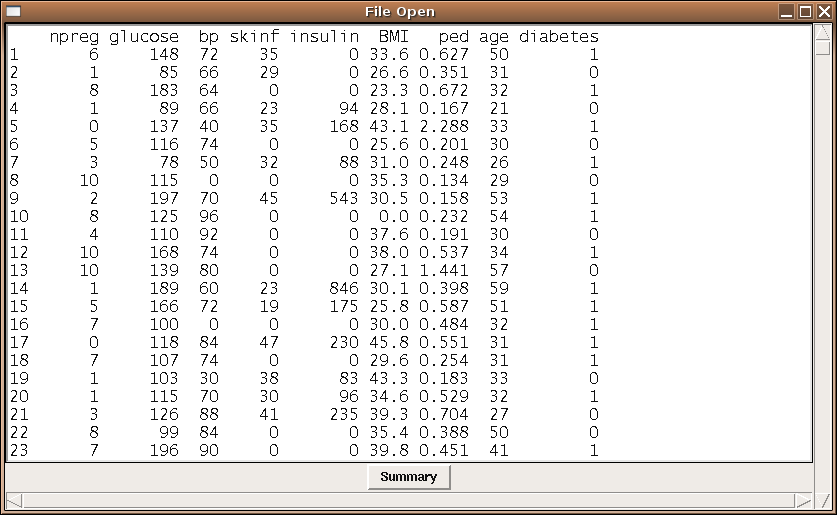
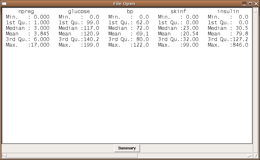
The first picture shows the file chooser (as displayed on a Linux system);
the second picture shows the diabetes data set displayed in a text window,
and the third picture shows the result of pressing the summary button.
7 Using Images with the tcltk package
The current version of tcl that ships with R allows you to display
images in your GUIs, but only if they are in GIF format. Fortunately,
it's very easy to change the format of images if they are, for example
JPEG or PNG files. On any SCF machine, the command:
mogrify -format gif *.jpg
will convert all the files ending in .jpg to files with
the same name, but in the GIF format. You can then use the .gif
files that are created to display in your GUI.
To use images with the tcltk library, first create a Tcl variable
representing the image with code like:
myimage = tclVar()
tcl("image","create","photo",myimage,file="picture.gif")
Next, create a tklabel using the image= argument
pointing to the tcl variable that holds the image:
img = tklabel(frame,image=myimage)
Like any other widget, you can change the image during the execution
of your program using the tkconfigure function. Suppose we have another
tcl variable called otherimage that has an image associated with it.
To change the img widget to display that image, use
tkconfigure(img,image=otherimage)
If you have many pictures, it will be more convenient to store the tcl image variables
in a list. Suppose the R list pics contains the full pathname of several
GIF files. (It's usually simplest to use setwd to change to the directory
where you're storing the GIF files, so that you only need to type their names, not
their full paths. The command
setwd(file.choose())
allows you to navigate to the directory with the GIF files.)
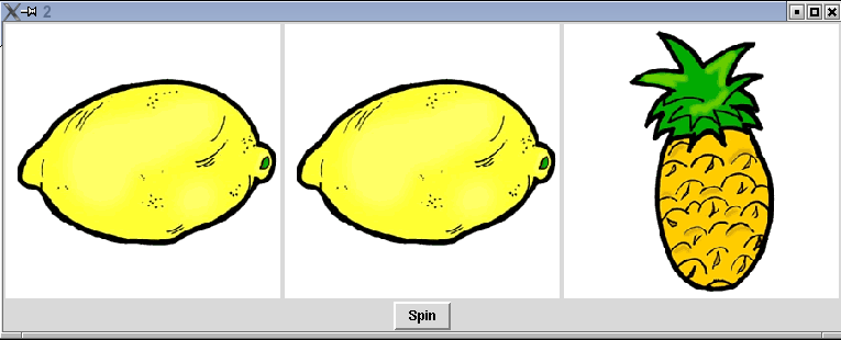
The following example displays pictures of three fruits, chosen from a list
of five. When the button is pressed, it uses tkconfigure to change
each picture many times, to give the illusion of a slot machine. Note the
use of sapply to create a list of images, regardless of the number
of images used.
require(tcltk)
pics = list.files('fruits',pattern='\\.gif$')
pics = paste('fruits/',pics,sep='')
n = length(pics)
theimages = sapply(pics,function(pic)
                             tcl("image","create","photo",tclVar(),file=pic))
spinner = function(...){
    for(i in 1:50){
        r = sample(1:n,size=3,replace=TRUE)
        tkconfigure(img1,image=theimages[[r[1]]])
        tkconfigure(img2,image=theimages[[r[2]]])
        tkconfigure(img3,image=theimages[[r[3]]])
	tcl('update')
        Sys.sleep(.07)
    }
}
top = tktoplevel()
f1 = tkframe(top)
f2 = tkframe(top)
r = sample(1:n,size=3,replace=TRUE)
img1 = tklabel(f1,image=theimages[[r[1]]])
img2 = tklabel(f1,image=theimages[[r[2]]])
img3 = tklabel(f1,image=theimages[[r[3]]])
tkpack(img1,side='left')
tkpack(img2,side='left')
tkpack(img3,side='left')
tkpack(tkbutton(f2,text='Spin',command=spinner),side='bottom')
tkpack(f1,side='top')
tkpack(f2,side='bottom')
A picture of the GUI before spinning is shown below
File translated from
TEX
by
TTH,
version 3.67.
On 19 Apr 2011, 12:06.