Spreadsheets and Databases
1 Spreadsheets
Spreadsheets, in particular the "xls" format used by Microsoft Excel, are
one of the most common (if not the most common) methods for transfering
data from one organization to another. When you download or receive a
spreadsheet, it's often a good idea to make sure that it really is a
spreadsheet. Comma-separated files, which are easily read into spreadsheet
programs, are often erroneously labeled "spreadsheets" or "Excel files",
and may even have an incorrect extension of ".xls".
In addition, Excel spreadsheets are often used to hold largely textual
information, so simply finding a spreadsheet that appears to contain data
can be misleading.
Furthermore, many
systems are configured to use a spreadsheet program to automatically open
files with an extension of ".csv", further adding to the confusion.
For many years, the only reliable way to read an Excel spreadsheet was with
Microsoft Excel, which is only available on Windows and Mac OS computers;
users on UNIX were left with no option other than finding a different computer.
In the last few years, a number of programs, notably gnumeric and
OpenOffice.org (usually
available through the ooffice command)
have been developed through careful reverse engineering to allow Unix users
the ability to work with these files.
To insure its advantage in the marketplace, Microsoft doesn't publish a
detailed description of exactly how it creates its spreadsheet files. There
are often "secret" ways of doing things that are only known to the
developers within Microsoft.
Reverse engineering means looking at the way a program handles different
kinds of files, and then trying to write a program that imitates what
the other program does.
The end result of all this is that there are several ways
to get the data from spreadsheet files into R.
Spreadsheets are organized as a collection of one or more sheets, stored in
a single file. Each of the sheets represents a rectangular display of rows
and columns, not unlike a data frame. Unfortunately, people often embed
text, graphics and pictures into spreadsheets, so it's not a good idea to
assume that a spreadsheet has the consistent structure of a data frame or
matrix, even if portions of it do appear to have that structure. In addition,
spreadsheets often have a large amount of header information (more than just
a list of variable names), sometimes making it challenging to figure out
the correct variable names to use for the different columns in the spreadsheet.
Our main concern will be in getting the information from the spreadsheet into
R:
we won't look at how to work with data within Excel.
If you are simply working with a single Excel spreadsheet, the easiest way
to get it into R is to open the spreadsheet with any compatible program, go
to the File menu, and select Save As. When the file selector dialog appears,
notice that you will be given an option of different file format choices,
usually through a drop down menu. Choose something like "Tab delimited text",
or "CSV (Comma separated values)". If any of the fields in the spreadsheet
contain commas, tab delimited is a better choice, but generally it doesn't
matter which one you use. Now, the file is (more or less) ready to
be read into R, using read.csv or read.delim. A very common
occurence is for fields stored in a spreadsheet to contain either single
or double quotes, in which case the quote= argument can be used to
make sure R understands what you want. Spreadsheets often arrange their
data so that there are a different number of valid entries on different lines,
which will confuse read.table; the fill= argument may be of
use in these cases. Finally, as mentioned previously, there are often multiple
descriptive lines of text at the top of a spreadsheet, so some experimentation
with the skip= argument to read.table may be necessary.
Alternatively, you can simply delete those lines from the file into which
you save the tab- or comma-delimited data.
As you can see, this is a somewhat time-consuming process which needs to be
customized for each spreadsheet. It's further complicated by the fact that
it only handles one sheet of a multi-sheet spreadsheet; in those cases the
process would need to be repeated for each sheet. If you need to read a
number of spreadsheets, especially ones where you need to access the data from
more than one sheet, you need to use a more programmable solution.
R provides several methods to read spreadsheets without having to save them as
tab- or comma-delimited files. The first is the read.xls function
in the gdata library. This function uses a Perl program (included
as part of the library), that converts the spreadsheet to a comma-separated
file, and then uses read.csv to convert it to a data frame.
In order for this library to work, perl must also be installed on
the computer that's running R. perl will be installed on virtually any
Unix-based computer (including Mac OSX), but will most likely not be on
most Windows computers (although once perl is installed on a Windows system, the
read.xls function will work with no problems). However there
is a Windows-only package , xlsReadWrite, available from CRAN
which can both read and write Excel files. (On other platforms, the
dataframes2xls package provides a write.xls function.)
Remember, for just one or two data tables from a spreadsheet, saving as a
tab- or comma-delimited
file and using the correct read.table variant will usually be the
easiest route.
Since read.xls does nothing more than convert the spreadsheet to
comma-separated form and then call read.csv, the guidelines for
using it are very similar to the normal use of read.csv. The
most useful feature of read.xls is that it accepts an optional
sheet= argument, allowing multiple sheets from a spreadsheet file to
be automatically read.
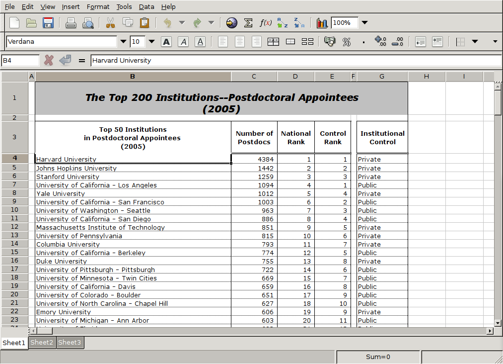
As a simple example, consider a spreadsheet with listings for the top 200
educational institutions in the US with respect to the number of postdoctoral
students, which I found at http://mup.asu.edu/Top200-III/2_2005_top200_postdoc.xls
Here's a view of how the data looks in the UNIX gnumeric spreadsheet:
 Here are the first few lines of the file created when I use File->Save As,
and choose the CSV format:
Here are the first few lines of the file created when I use File->Save As,
and choose the CSV format:
"The Top 200 Institutions--Postdoctoral Appointees
(2005)",,,,,
,,,,,
"Top 50 Institutions
in Postdoctoral Appointees
(2005)","Number of Postdocs","National Rank","Control Rank",,"Institutional
Control"
"Harvard University",4384,1,1,,Private
"Johns Hopkins University",1442,2,2,,Private
"Stanford University",1259,3,3,,Private
"University of California - Los Angeles",1094,4,1,,Public
"Yale University",1012,5,4,,Private
"University of California - San Francisco",1003,6,2,,Public
"University of Washington - Seattle",963,7,3,,Public
"University of California - San Diego",886,8,4,,Public
"Massachusetts Institute of Technology",851,9,5,,Private
"University of Pennsylvania",815,10,6,,Private
"Columbia University",793,11,7,,Private
"University of California - Berkeley",774,12,5,,Public
While the data itself looks fine, it's unlikely that the header information
will be of much use. Since there are 7 header lines, I could use the
following statements to read the data into R:
> fromcsv = read.csv('2_2005_top200_postdoc.csv',header=FALSE,skip=7,stringsAsFactors=FALSE)
> dim(fromcsv)
[1] 206   6
> head(fromcsv)
                                        V1   V2 V3 V4 V5      V6
1                       Harvard University 4384  1  1 NA Private
2                 Johns Hopkins University 1442  2  2 NA Private
3                      Stanford University 1259  3  3 NA Private
4   University of California - Los Angeles 1094  4  1 NA  Public
5                          Yale University 1012  5  4 NA Private
6 University of California - San Francisco 1003  6  2 NA  Public
The fifth column can be removed (take a look at the spreadsheet to see why),
and we should supply some names to the spreadsheet. One problem with this
spreadsheet is that it repeats its header information several times part way
through the spreadsheet. These lines will have to be removed manually.
The can be identified by the fact that the sixth variable should be either
Public or Private, and could be eliminated as follows:
> fromcsv = fromcsv[fromcsv$V6 %in% c('Public','Private'),]
The fifth variable can be removed by setting it to NULL, and the
columns can be named.
> fromcsv$V5 = NULL
> names(fromcsv) = c('Institution','NPostdocs','Rank','ControlRank','Control')
Finally, a check of the columns shows that, because of the header problem,
the numeric variables explicitly need to be converted:
> sapply(fromcsv,class)
Institution   NPostdocs        Rank ControlRank     Control
"character" "character" "character" "character" "character"
> fromcsv[,c(2,3,4)] = sapply(fromcsv[,c(2,3,4)],as.numeric)
A similar procedure could be carried out with read.xls, although it
might take some experimentation with skip= to make things work
properly. The only other difference between read.xls and read.csv
for this example is that a space mysteriously appeared at the end of one of the
variables when using read.xls:
library(gdata)
fromreadxls = read.xls('2_2005_top200_postdoc.xls',stringsAsFactors=FALSE,header=FALSE,skip=2)
fromreadxls = fromreadxls[-1,-c(1,6)]
fromreadxls$V7 = sub(' $','',fromreadxls$V7)
fromreadxls = fromreadxls[fromreadxls$V7 %in% c('Public','Private'),]
fromreadxls[,c(2,3,4)] = sapply(fromreadxls[,c(2,3,4)],as.numeric)
names(fromreadxls) = c('Institution','NPostdocs','Rank','ControlRank','Control')
2 Databases
A database is a collection of data, usually with some information (sometimes called
metadata) about how the data is organized. But many times when people refer to a
database, they mean a database server, which is similar to a web server, but responds
to requests for data instead of web pages.
By far the most common type of database server is known a a relational database
management system (RDBMS), and the most common way of communicating with such a database
is a language known as SQL, which is an acronym for Structured Query Language.
Some examples of database systems that use SQL to communicate with an RDBMS include
Oracle, Sybase, Microsoft SQL Server, SQLite, MySQL and Postgres. While there is an SQL
standard, each database manufacturer provides some additional features, so SQL that
works with one database is not guaranteed to work on another. We'll try to stick to
aspects of SQL that should be available on most SQL based systems.
A Database consists of one or more tables, which are generally stored as files on the
computer that's running the DBMS. A table is a rectangular array, where each row
represents an observation, and each column represents a variable. Most databases
consists of several tables, each containing information about one aspect of the data.
For example, consider a database to hold information about the parts needed to build
a variety of different products. One way to store the information would be to have
a data table that had the part id, its description, the supplier's name, and the
cost of the part. An immediate problem with this is scheme concerns how we could store
information about the relation between products and parts. Furthermore, if one supplier
provided many different parts, redundant information
about suppliers would be repeated many times in the data table. In the 1970s when
database technology was first being developed, disk and memory space were limited and
expensive, and organizing data in this way was not very efficient, especially as the
size of the data base increased. In the late 1970s, the idea of a relational database
was developed by IBM, with the first commercial offering coming from a company which is
now known as Oracle. Relational database design is governed by a principle known as
normalization. While entire books are devoted to the subject, the basic idea of normalization
is to try and remove redundancy as much as possible when creating the tables that make up
a data base. Continuing the parts example, a properly normalized database to hold the
parts information would consist of four tables. The first would contain a part id to uniquely
identify the part, its description, price and an id to identify the supplier. A second table
would contain the supplier codes and any other information about the supplier. A third table
would contain product ids and descriptions, while the final table would have one record for
each part used in each product, stored as pairs of product id and part id.
The variables that link together the different databases are refered to as keys, or sometimes
foreign keys. Clearly, making sure that there are keys to link information from one table to
another is critical to the idea of a normalized data base.
This allows large
amounts of information to be stored in manageably sized tables which can be modified and updated
without having to change all of the information in all of the tables. Such tables will be
efficient in the amount of disk and memory resources that they need, which was critical at the
time such databases were developed. Also critical to this scheme is a fast and efficient way of
joining together these tables so that queries like "Which suppliers are used for product xyz?"
or "What parts from Acme Machine Works cost between $2 and $4" or "What is the total cost of
the parts needed to make product xyz?". In fact, for many years the only programs that were
capable of combining data from multiple sources were RDBMSs.
We're going to look at the way the SQL language is used to extract information from RDBMSs,
specifically the open source SQLite data base (http://sqlite.org)
(which doesn't require a database server), and
the open source MySQL data base (http://www.mysql.com) which does.
In addition we'll see how to do typical database operations in R,
and how to access a database using SQL from inside of R.
One of the first questions that arises when thinking about databases is "When should I
use a database?" There are several cases where a database makes sense:
- The only source for the data you need may be an existing database.
-
The data you're working with changes on a regular basis, especially if it can
potentially be changed by many people. Database servers (like most other servers)
provide concurrency, which takes care of problems that might otherwise arise if
more than one person tries to access or modify a database at the same time.
-
Your data is simply too big to fit into the computer's memory, but if you could
conveniently extract just the parts you need, you'd be able to work with the data.
For example, you may have hundreds of variables, but only need to work with a small
number at at time, or you have tens of thousands of observations, but only need to work
with a few thousand at a time.
One of the most important uses of databases in the last ten years has been as back
ends to dynamic web sites. If you've ever placed an order online, joined an online
discussion community, or gotten a username/password combination to access web
resources, you've most likely interacted with a database. In addition both the
Firefox and Safari browsers us
SQLite databases to store cookies, certificates, and other information.
There are actually three parts to a RDBMS system: data definition, data access, and
privelege management. We're only going to look at the data access aspect of databases;
we'll assume that a database is already available, and that the administrator of the
database has provided you with access to the resources you need. You can communicate
with a database in at least three different ways:
- You can use a command line program that will display its results in a way similar to
the way R works: you type in a query, and the results are displayed.
-
You can use a graphical interface (GUI) that will display the results and give you the
option to export them in different forms, such as a comma-separated data file. One
advantage to these clients is that they usually provide a display of the available
databases, along with the names of the tables in the database and the names of the columns
within the tables.
-
You can use a library within R to query the database and return the results of the query
into an R data frame. For use with MySQL library, the RMySQL library is available for
download from CRAN; for SQLite, the RSQLite package is available. When you install either,
the DBI
library, which provides a consistent interface to different databases, will also be installed.
It's very important to understand that SQL is not a programming language - it's said
to be a declarative language. Instead of solving problems by writing a series of
instructions or putting together programming statements into functions, with SQL you
write a single statement (query) that will return some or all of the records from a
database. SQL was designed to be easy to use for non-programmers, allowing them to
present queries to the database in a language that is more similar to a spoken language
than a programming language. The main tool for data access is the select statement.
Since everything needs to be done with this single statement, descriptions of its syntax
can be quite daunting. For example, here's an example that shows some of the important features
of the select statement:
SELECT columns or computations
       FROM table
       WHERE condition
       GROUP BY columns
       HAVING condition
       ORDER BY column [ASC | DESC]
       LIMIT offset,count;
(The keywords in the above statement can be typed in upper or lower case, but I'll generally
use upper case to remind us that they are keywords.) MySQL is case sensistive to table and
column names, but not for commands. SQLite is not case sensitive at all.
SQL statements always end with a semi-colon,
but graphical clients and interfaces in other languages sometimes don't require the semi-colon.
Fortunately, you rarely need to use all of these commands in a single query. In fact,
you may be able to get by knowing just the command that returns all of the information
from a table in a database:
SELECT * from table;
3 Working with Databases
When you're not using a graphical interface, it's easy to get lost in a database considering
that each database can hold multiple tables, and each table can have multiple columns. Three
commands that are useful in finding your way around a database are:
| MySQL | SQLite |
| SHOW DATABASES; | .databases |
| SHOW TABLES IN database; | .tables |
| SHOW COLUMNS IN table; | pragma table_info(table) |
| DESCRIBE table; | .schema table |
For use as an example, consider a database to keep track of a music collection, stored as
an SQLite database in the file albums.db. (You can download the database from
http://www.stat.berkeley.edu/~spector/s133/albums.db) We can use the commands just shown to see how the
database is organized. Here, I'm using the UNIX command-line client called sqlite3:
springer.spector$ sqlite3 albums.db
SQLite version 3.4.2
Enter ".help" for instructions
sqlite> .mode column
sqlite> .header on
sqlite> .tables
Album   Artist  Track
sqlite> .schema Album
CREATE TABLE Album
( alid INTEGER,
	aid REAL,
	title TEXT
);
CREATE INDEX jj on Album(alid);
sqlite> .schema Artist
CREATE TABLE Artist
( aid REAL,
	name TEXT
);
CREATE INDEX ii on Artist(aid);
sqlite> .schema Track
CREATE TABLE Track
( alid INTEGER,
	aid REAL,
	title TEXT,
	filesize INTEGER,
	bitrate REAL,
	length INTEGER
);
Studying these tables we can see that the organization is as follows: each track
in the Track table
is identified by an artist id (aid) and an album id (alid). To
get the actual names of the artists, we can link to the Artist database
through the aid key; to get the names of the albums, we can link to the
Album table through the alid key. These keys are integers, which
don't take up very much space; the actual text of the album title or artist's name
is stored only once in the table devoted to that purpose. (This is the basic
principle of normalization that drives database design.) The first thing to notice
in schemes like this is that the individual tables won't allow us to really see
anything iteresting, since they just contain keys, not actual values; to get interesting
information, we need to join together multiple tables. For example, let's say we want
a list of album titles and artist names. We want to extract the Name from the
Artist table and combine it with Title from the Album table,
based on a matching value of the aid variable:
sqlite> .width 25 50
sqlite> SELECT Artist.name, Album.title FROM Artist, Album WHERE Artist.aid = Album.aid;
name                       title
-------------------------  --------------------------------------------------
Jimmy McGriff              100% Pure Funk
Jimmy McGriff              A Bag Full Of Soul
Jimmy McGriff              Cherry
Jimmy McGriff              Countdown
Jimmy McGriff              Electric Funk
Jimmy McGriff              The Starting Five
Tiny Parham                1926-1929
Tiny Parham                1929-1940
Jimmie Noone               1928-1929
Ethel Waters, Benny Goodm  1929-1939
Cab Calloway               1930-1931
Cab Calloway               Best Of Big Bands
                         . . .
Queries like this are surprisingly fast - they are exactly what the database has been designed
and optimized to acheive.
File translated from
TEX
by
TTH,
version 3.67.
On 4 Mar 2009, 15:35.