Analysis of Variance
1 Analysis of Variance
In its simplest form, analysis of variance (often abbreviated as ANOVA), can be
thought of as a generalization of the t-test, because it allows us to test the
hypothesis that the means of a dependent variable are the same for several groups,
not just two as would be the case when using a t-test. This type of ANOVA is
known as a one-way ANOVA.
In cases where there are multiple classification variables, more complex ANOVAs
are possible. For example, suppose we have data on test scores for students from
four schools, where three different teaching methods were used. This would
describe a two-way ANOVA. In addition to asking whether the means for the
different schools were different from each other, and whether the means for the
different teaching methods were different from each other, we could also
investigate whether the differences in teaching methods were different depending
on which school we looked at. This last comparison is known as an interaction,
and testing for interactions is one of the most important uses of analysis of
variance.
Before getting to the specifics of ANOVA, it may be useful to ask why we
perform an analysis of variance if our interest lies in the differences between
means.
If we were to concentrate on the differences between the means, we would have
many different comparisons to make, and the number of comparisons would increase
as we increased the number of groups we considered. Thus, we'd need different
tests depending on how many groups we were looking at. The reasoning behind
using variance to test for differences in means is based on the following idea:
Suppose we have several groups of data, and we calculate their variance in two
different ways. First, we put together all the data, and simply calculate its
variance disregarding the groups from which the data arose.
In other words, we evaluate the deviations of the data relative to overall mean
of the entire data set.
Next, we calculate
the variance by adding up the deviations around the mean of each of the groups.
The idea of analysis of variance is that if the two variance calculations give
us very similar results, then each of the group means must have been about the
same, because using the group means to measure variation didn't result in a big
change than from using the overall mean. But if the overall variance is bigger than
the variance calculated using the group means, then at least one of the group
means must have been different from the overall mean, so it's unlikely that the
means of all the groups were the same. Using this approach, we only need to
compare two values (the overall variance, and the variance calculated using each
of the group means) to test if any of the means are different, regardless of
how many groups we have.
To illustrate how looking at variances can tell us
about differences in means, consider a data set with
three groups, where the mean of the first group is
3, and the mean for the other groups is 1. We can
generate a sample as follows:
> mydf = data.frame(group=rep(1:3,rep(10,3)),x=rnorm(30,mean=c(rep(3,10),rep(1,20))))
Under the null hypothesis of no differences among the means,
we can center each set of data by the appropriate group mean,
and then compare the data to the same data centered by
the overall mean. In R, the ave function will return
a vector the same length as its' input, containing summary statistics
calculated by grouping variables. Since ave accepts an
unlimited number of grouping variables, we must identify the function
that calculates the statistic as the FUN= argument. Let's
look at two histograms of the data, first centered by the overall mean,
and then by the group means. Recall that under the null hypothesis,
there should be no difference.
> ovall = mydf$x - mean(mydf$x)
> group = mydf$x - ave(mydf$x,mydf$group,FUN=mean)
> par(mfrow=c(2,1))
> hist(ovall,xlim=c(-2,2.5))
> hist(group,xlim=c(-2,2.5))
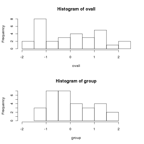 Notice how much more spread out the data is when we centered by the
overall mean. To show that this isn't a trick, let's generate some
data for which the means are all equal:
Notice how much more spread out the data is when we centered by the
overall mean. To show that this isn't a trick, let's generate some
data for which the means are all equal:
> mydf1 = data.frame(group=rep(1:3,rep(10,3)),x=rnorm(30))
> ovall = mydf1$x - mean(mydf1$x)
> group = mydf1$x - ave(mydf1$x,mydf1$group,FUN=mean)
> par(mfrow=c(2,1))
> hist(ovall,xlim=c(-2.5,3.2))
> hist(group,xlim=c(-2.5,3.2))
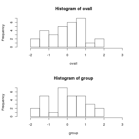 Notice how the two histograms are very similar.
To formalize the idea of a one-way ANOVA, we have a data set with a dependent
variable and a grouping variable. We assume that the observations are
independent of each other, and the errors (that part of the data not explained
by an observation's group mean) follow a normal distribution with the same
variance for all the observations. The null hypothesis states that the means
of all the groups are equal, against an alternative that at least one of the means
differs from the others. We can test the null hypothesis by taking the ratio
of the variance calculated in the two ways described above, and comparing it to
an F distribution with appropriate degrees of freedom (more on that later).
In R, ANOVAs can be performed with the aov command. When you are
performing an ANOVA in R, it's very important that all of the grouping variables
involved in the ANOVA are converted to factors, or R will treat them as if they
were just independent variables in a linear regression.
As a first example, consider once again the wine data frame. The
Cultivar variable represents one of three different varieties of wine
that have been studied. As a quick preliminary test, we can examine a dotplot
of Alcohol versus Cultivar:
Notice how the two histograms are very similar.
To formalize the idea of a one-way ANOVA, we have a data set with a dependent
variable and a grouping variable. We assume that the observations are
independent of each other, and the errors (that part of the data not explained
by an observation's group mean) follow a normal distribution with the same
variance for all the observations. The null hypothesis states that the means
of all the groups are equal, against an alternative that at least one of the means
differs from the others. We can test the null hypothesis by taking the ratio
of the variance calculated in the two ways described above, and comparing it to
an F distribution with appropriate degrees of freedom (more on that later).
In R, ANOVAs can be performed with the aov command. When you are
performing an ANOVA in R, it's very important that all of the grouping variables
involved in the ANOVA are converted to factors, or R will treat them as if they
were just independent variables in a linear regression.
As a first example, consider once again the wine data frame. The
Cultivar variable represents one of three different varieties of wine
that have been studied. As a quick preliminary test, we can examine a dotplot
of Alcohol versus Cultivar:
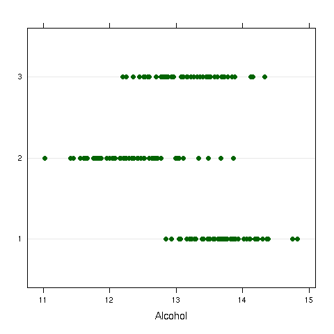 It does appear that there are some differences, even though there is overlap.
We can test for these differences with an ANOVA:
It does appear that there are some differences, even though there is overlap.
We can test for these differences with an ANOVA:
> wine.aov = aov(Alcohol~Cultivar,data=wine)
> wine.aov
Call:
   aov(formula = Alcohol ~ Cultivar, data = wine)

Terms:
                Cultivar Residuals
Sum of Squares  70.79485  45.85918
Deg. of Freedom        2       175

Residual standard error: 0.5119106
Estimated effects may be unbalanced
> summary(wine.aov)
             Df Sum Sq Mean Sq F value    Pr(>F)
Cultivar      2 70.795  35.397  135.08 < 2.2e-16 ***
Residuals   175 45.859   0.262
---
Signif. codes:  0 '***' 0.001 '**' 0.01 '*' 0.05 '.' 0.1 ' ' 1
The summary function displays the ANOVA table, which is similar
to that produced by most statistical software. It indicates that the
differences among the means are statistically significant. To see the
values for the means, we can use the aggregate function:
> aggregate(wine$Alcohol,wine['Cultivar'],mean)
  Cultivar        x
1        1 13.74475
2        2 12.27873
3        3 13.15375
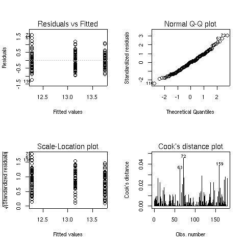
The default plots from an aov object are the same as those for
an lm object. They're displayed below for the Alcohol/Cultivar ANOVA we just calculated:
File translated from
TEX
by
TTH,
version 3.67.
On 26 Apr 2010, 15:23.