Once you get more advanced using R, you will inevitably want to write your own functions, if only to save time doing something you do repetitively. Generally, the function writing is straightforward. I give some basic over view and I give a lot of personal “tips” that I have found confusing at times.
For understanding functions, in particular, it will be very hard to understand if you do not follow along and make sure you understand what the toy examples are doing. Also, the functions are toy examples to explain a point – unless otherwise stated I don’t promise that they are efficient and certainly have no claims to actually being useful!
You define a function in R using the command function. The format is
myfun<-function(x,y,z=2){

}
where x,y, and z are the user-supplied variables that the function needs to run the code. Note you can easily define default values by giving those values in your declaration as I did with z=2.
The following function returns the mean of the data, with argument x required to be given by the user. The function return returns the results to the user.
mysum<-function(x){
    m<-mean(x)
    return(m)
}
library(MASS)
data(UScereal)
mysum(UScereal$potassium)
## [1] 159.1197I can make this more fancy, by returning the mean and standard deviation, as a list
mysum<-function(x){
    m<-mean(x)
    s<-sd(x)
    return(list(mean=m,sd=s))
}
library(MASS)
data(UScereal)
mysum(UScereal$potassium)
## $mean
## [1] 159.1197
##
## $sd
## [1] 180.2886Now, I am going to adapt it to optionally give a upper and lower 95% confidence interval limits if the argument conf.inv=TRUE. Note I give a default value for the value of conf.inv, but x must be supplied by the user. I will use if statements to return different results depending on conf.inv
mysum<-function(x, conf.inv=TRUE){
    m<-mean(x)
    s<-sd(x)
    if(conf.inv==TRUE){
        n<-length(x)
        uppconf<-m+2*sd(x)/sqrt(n)
        lowconf<-m-2*sd(x)/sqrt(n)
        return(list(mean=m,sd=s,uppconf=uppconf,lowconf=lowconf))
    }
    else return(list(mean=m,sd=s))
}
library(MASS)
data(UScereal)
mysum(UScereal$potassium)
## $mean
## [1] 159.1197
##
## $sd
## [1] 180.2886
##
## $uppconf
## [1] 203.8438
##
## $lowconf
## [1] 114.3957If you want to pass along commands to another function, you can add ... to your function call:
# originally will give NAs
mysum(c(1,2,3,4,NA))
## $mean
## [1] NA
##
## $sd
## [1] NA
##
## $uppconf
## [1] NA
##
## $lowconf
## [1] NA# Now can pass na.rm to all the functions via ...
mysum<-function(x, conf.inv=T,...){
m<-mean(x,...)
if(conf.inv==T){
n<-length(x[complete.cases(x)])
uppconf<-m+2*sd(x,...)/sqrt(n)
lowconf<-m-2*sd(x,...)/sqrt(n)
return(list(mean=m,sd=sd(x),uppconf=uppconf,lowconf=lowconf))
}
else return(list(mean=m,sd=sd(x,...)))
}
mysum(c(1,2,3,4,NA),na.rm=TRUE,conf.inv=FALSE)## $mean
## [1] 2.5
##
## $sd
## [1] 1.290994Basic programming functions are,
These are standard function controls used as in pretty much any programming language. One nice feature of for is that the index does not have to be from 1 to n.
myindex<-seq(1,5,by=2) #odd numbers from 1 to 5
## Way to do it going over 1:3 (length of myindex)
for(i in 1:3){
    print(UScereal[myindex[i],1:3])
}
## mfr calories protein
## 100% Bran N 212.1212 12.12121
## mfr calories protein
## All-Bran with Extra Fiber K 100 8
## mfr calories protein
## Apple Jacks K 110 2## Simpler, go over myindex directly
for(i in myindex){
print(UScereal[i,1:3])
}## mfr calories protein
## 100% Bran N 212.1212 12.12121
## mfr calories protein
## All-Bran with Extra Fiber K 100 8
## mfr calories protein
## Apple Jacks K 110 2(but see Tips below, about using for)
You can comment your code using the # symbol. stop and warning are functions that allow user to check that certain conditions are satisfied.
myfunc<-function(x){
    if(!(is.matrix(x)|is.data.frame(x))) stop("x must be matrix")
    if(is.data.frame(x)){
        x<-data.matrix(x)
        warning("Converting data.frame to matrix")
    }
    t(x)%*%x
}
myfunc(UScereal[,2:3])
## Warning in myfunc(UScereal[, 2:3]): Converting data.frame to matrix## calories protein
## calories 1700279.28 43226.774
## protein 43226.77 1328.969myfunc(c(1,23))## Error in myfunc(c(1, 23)): x must be matrixSelf-explanatory logical commands for testing about objects(see Tips for more about logical commands):
Others:
missing: test if parameter was defined by user or given a default valuehasArg: like !missing(x), but will check the “…” parameters passed alongmatch.arg: try to match the character string the user gave for a parameter with a list of possible alternatives – useful so user doesn’t have to give the whole string and also has good error handling if the user gives an unacceptable valuerequire: loads a package if not already loaded that is need for that function to runcat: A good way to print to the screen – much nicer looking than ttprint` for giving messages to the useron.exit: function will perform actions before it exits – useful for resetting changes to par in plotting functions, for exampleYou can time how long something will take with system.time.
system.time(for (i in 1:1000) mad(runif(500)))## user system elapsed
## 0.232 0.013 0.245The third element tells you the total elapsed time to run the code in parenthesis. It will, of course vary depending on your machine.
Often, you may find that you want to see how a R program works or make your own version of it. In general, you can see a function by typing its name at the prompt:
weighted.mean## function (x, w, ...)
## UseMethod("weighted.mean")
## <bytecode: 0x7f8c6513a0f0>
## <environment: namespace:stats>If you use variables in your function that are not defined in your function, R will go and look for them. What I mean, is that if you say sum(x), R will first to see if x was defined somewhere in the current function, and if not it will progressively search back to find a x. So if you have an x that you defined in your normal workspace, R will use it if there is no other definition. For example:
rm(x) #make sure you don't have x defined already.
xfunc<-function(){print(x)}
xfunc()
## Error in print(x): object 'x' not foundx<-c(2,3) #now define a value x in your workspace
xfunc()## [1] 2 3This can be quite useful actually, but is not intuitive for people who have programmed in other languages. And it can be quite dangerous if you have objects with common names like n or x that you forgot to define in your function – if they exist in your workspace then R will use those with no warning!
This can actually be quite tricky to discover if you have a long function and you forgot what name you used. Another common time this comes up is if you are starting with code that you tried out on a small data example and you forgot to change the names somewhere. Unbeknownst to you, R is using only that specific dataset set in your workspace, rather than the dataset the user gave to the function!
apply versus forNote that for loops are generally slow in R, and using apply or sapply is considered preferable if the function is not actually recursive. This really comes in to play if you have {} large for-loops or large data sets. For normal operations, you probably won’t notice, so don’t worry about this too much, and just try to get your function working! But most experience R users use apply type functions regularly, so it’s still pretty important to be able to understand the functions if you want to be able to read other people’s functions. Also the code is a lot nicer to read once you are use to it.
For example, the following code that finds the upper confidence interval for the 2nd, 4th, and 8th column of UScereal
my.ind<-c(2,4,8)
x<-vector(length=length(my.ind))
n<-nrow(UScereal)
for(i in my.ind ){ #note how I don't have to make i=1,2,3, etc.
      x[i]<-mean(UScereal[,i])+
            2*sd(UScereal[,i])/sqrt(n)
  }
x
## [1] 0.000000 164.890738 0.000000 1.831168 NA NA
## [7] NA 11.498387could be written as
x<-apply(UScereal[,my.ind],2,function(y){
          mean(y)+2*sd(y)/sqrt(length(y))})
x
## calories fat sugars
## 164.890738 1.831168 11.498387If the function is already defined (by you or by R), then apply is even easier:
out<-apply(UScereal[,my.ind],1,mean)
head(out)
## 100% Bran All-Bran
## 77.77778 76.76768
## All-Bran with Extra Fiber Apple Cinnamon Cheerios
## 33.33333 54.22222
## Apple Jacks Basic 4
## 41.33333 62.22222finds the row means across the columns defined in my.ind.
Note that generally R automatically changes a 1-dimensional matrix into a vector, and these objects are not treated the same. In particular, apply requires matrices.
myMatrix<-matrix(rnorm(4),ncol=2,nrow=2)
Numb<-myMatrix[1,]
Numb
## [1] 0.85195866 0.08023243apply(Numb,1,sum)## Error in apply(Numb, 1, sum): dim(X) must have a positive lengthapply(matrix(Numb,nrow=1),1,sum)## [1] 0.9321911This is really unfortunate behavior, from the point of view of programming. Namely if you don’t know if a matrix you will be using might sometimes be 1-dimensional, then you have to be very careful since it will probably be turned into a vector by R. If you are using apply, then you should be ok if you make sure that you always have 1-dimensional matrices rather than vectors. In particularly, if you are indexing a matrix, you should always say drop=FALSE to tell R not to convert a 1-dim matrix to a vector.
The following example is a function that very simply gives the median of the rows of the matrix mat as given in the parameter row.ind, using the drop=FALSE option to guarantee that the subsetting of columns doesn’t reduce the matrix to a vector
cereal.mat<-data.matrix(UScereal[,2:8])
#wrong
a.fun<-function(mat,col.ind){
    colMed<-apply(mat[,col.ind],2,median)
    return(colMed)
}
a.fun(UScereal,2:3)
## calories protein
## 134.3284 3.0000a.fun(UScereal,2) ## Error in apply(mat[, col.ind], 2, median): dim(X) must have a positive length#correct
a.fun<-function(mat,col.ind){
colMed<-apply(mat[,col.ind,drop=FALSE],2,median)
return(colMed)
}
a.fun(UScereal,2) ## calories
## 134.3284data.frame is a list, not matrixEven though data frames generally act like matrices, they are actually simple lists. Therefore sometimes you need to them to be numeric, the simplest case being matrix operations:
t(UScereal[,2:8])%*%UScereal[,2:8]## Error in t(UScereal[, 2:8]) %*% UScereal[, 2:8]: requires numeric/complex matrix/vector argumentsThis can also give unexpected results for sapply sometimes. The following has a simple function of i that just returns UScereal[i:(i+2),1:3] – a small data.frame. When using lapply on i=1,2,3, it returns a list with each element consisting of the small data frame returned by the function:
little.func<-function(i){UScereal[i:(i+2),1:3]}
lapply(1:3,little.func)
## [[1]]
## mfr calories protein
## 100% Bran N 212.1212 12.12121
## All-Bran K 212.1212 12.12121
## All-Bran with Extra Fiber K 100.0000 8.00000
##
## [[2]]
## mfr calories protein
## All-Bran K 212.1212 12.121212
## All-Bran with Extra Fiber K 100.0000 8.000000
## Apple Cinnamon Cheerios G 146.6667 2.666667
##
## [[3]]
## mfr calories protein
## All-Bran with Extra Fiber K 100.0000 8.000000
## Apple Cinnamon Cheerios G 146.6667 2.666667
## Apple Jacks K 110.0000 2.000000If UScereal were a matrix, then the output of little.func would be a matrix and if I used sapply instead of lapply then the answer would be squashed into a matrix:
sapply(1:3,function(i){data.matrix(UScereal)[i:(i+2),1:3]})## [,1] [,2] [,3]
## [1,] 3.00000 2.000000 2.000000
## [2,] 2.00000 2.000000 1.000000
## [3,] 2.00000 1.000000 2.000000
## [4,] 212.12121 212.121210 100.000000
## [5,] 212.12121 100.000000 146.666670
## [6,] 100.00000 146.666670 110.000000
## [7,] 12.12121 12.121212 8.000000
## [8,] 12.12121 8.000000 2.666667
## [9,] 8.00000 2.666667 2.000000Instead I get a very odd answer, and this is because sapply is trying to squash little lists together:
temp<-sapply(1:3,little.func)
temp
## [,1] [,2] [,3]
## mfr factor,3 factor,3 factor,3
## calories Numeric,3 Numeric,3 Numeric,3
## protein Numeric,3 Numeric,3 Numeric,3temp[1,1:2]## [[1]]
## [1] N K K
## Levels: G K N P Q R
##
## [[2]]
## [1] K K G
## Levels: G K N P Q RIn if statements, you should use any, all for robust programing.
y<-"yes"
x<-c(1,3)
if(x>2) print(y) else print(x);
## Warning in if (x > 2) print(y) else print(x): the condition has length > 1
## and only the first element will be used## [1] 1 3if(any(x>2)) print(y) else print(x);## [1] "yes"if(all(x>2)) print(y) else print(x);## [1] 1 3If you are making random objects to test your function or for other purpose, use set.seed to guarantee you get the same random object each time.
plotinvisible for a function to return a value only if it is assigned to a new variable; good for returning the coordinates, etc. only if asked... by using the defaults in par. This means that if the user changes the settings in par, your function will respond nicely.R does not have great debugging mechanisms and the error messages are … cryptic. Here are a couple of things that can be helpful
Save your function by itself in a text/.R file. Then when you want to load it into R, use the source command. This reads the file and executes the file. For a file with just a function, this will load your function or changes, and most importantly, will tell you the line number of a syntax error.
If you are calling functions within functions, as we did in calling mean and sd, traceback() tells you what function had the error
fun1<-function(x){table(x)}
fun2<-function(x){sum(x)}
myerror<-function(){
    x<-c("yes","no")
    fun1(x)
    fun2(x)
}
myerror()
## Error in sum(x): invalid 'type' (character) of argumenttraceback()## No traceback availableThere are several functions that are suppose to help debug your function. I find the most useful is debug. This allows you go along with the function and figure out what the problem is. My function is suppose to both subtract the mean of each column and each row (there’s a function that centers matrices, by the way, sweep or scale)
myCentered<-function(x){
    rsum<-apply(x,1,mean)
    rcentered<-x-rsum
    csum<-apply(x,2,mean)
    ccentered<-x-csum
    return(list(row=rcentered,col=ccentered))
    }
set.seed(39805)
mat<-matrix(sample(1:100,size=15),nrow=3,ncol=5)
myCentered(mat)
## $row
## [,1] [,2] [,3] [,4] [,5]
## [1,] 35.8 41.8 -57.2 -28.2 7.8
## [2,] -14.0 33.0 -39.0 9.0 11.0
## [3,] -21.0 8.0 31.0 -1.0 -17.0
##
## $col
## [,1] [,2] [,3] [,4] [,5]
## [1,] 39.00000 52.00000 -81.33333 -25.33333 33.00000
## [2,] -46.33333 27.66667 -22.00000 4.00000 13.00000
## [3,] 2.00000 9.00000 39.00000 -27.33333 -16.33333There’s no error, just not what I was wanting – the row centering worked, but the column centering didn’t (a matrix minus a vector works column-wise, not row-wise; so x-csum doesn’t subtract off csum from each row, even though x-rsum does subtract rsum from each column).
I can use debug go into the function and try it as it is working. Namely, R pauses and prints each command and waits to execute it until you ask it to. To get R to execute the next line, hit “return” or type “n”. While it’s paused, you can just type in what you want within the operation of the function using the objects within the function. This is very helpful with large functions. This is interactive, but I give the output from a debugging below. Try to follow along with the code below to get the idea.
> debug(myCentered)
> myCentered(mat)
> myCentered(mat)
debugging in: myCentered(mat)
debug at #1: {
    rsum <- apply(x, 1, mean)
    rcentered <- x - rsum
    csum <- apply(x, 2, mean)
    ccentered <- x - csum
    return(list(row = rcentered, col = ccentered))
}
Browse[2]> n
debug at #2: rsum <- apply(x, 1, mean)
Browse[2]> n
debug at #3: rcentered <- x - rsum
Browse[2]> n
debug at #4: csum <- apply(x, 2, mean)
Browse[1]> csum #I try to look at my object too soon
Error: Object "csum" not found
Browse[2]> n
debug at #5: ccentered <- x - csum
Browse[2]> csum #now its there
[1] 55.00000 82.33333 33.00000 48.00000 55.33333
Browse[2]>  x
     [,1] [,2] [,3] [,4] [,5]
[1,]   94  100    1   30   66
[2,]   36   83   11   59   61
[3,]   35   64   87   55   39
Browse[2]> x-csum  # So I see this subtracts off across rows...
          [,1]     [,2]      [,3]      [,4]      [,5]
[1,]  39.00000 52.00000 -81.33333 -25.33333  33.00000
[2,] -46.33333 27.66667 -22.00000   4.00000  13.00000
[3,]   2.00000  9.00000  39.00000 -27.33333 -16.33333
Browse[2]> t(x)-csum # the right answer, but transposed...
          [,1]        [,2]      [,3]
[1,]  39.00000 -19.0000000 -20.00000
[2,]  17.66667   0.6666667 -18.33333
[3,] -32.00000 -22.0000000  54.00000
[4,] -18.00000  11.0000000   7.00000
[5,]  10.66667   5.6666667 -16.33333
Browse[2]> t(t(x)-csum) #there we go, now I can fix it with this code
     [,1]        [,2] [,3] [,4]       [,5]
[1,]   39  17.6666667  -32  -18  10.666667
[2,]  -19   0.6666667  -22   11   5.666667
[3,]  -20 -18.3333333   54    7 -16.333333
Browse[2]> Q #get me out of here without finishing
> undebug(myCentered)#Turns off the debuggingSee if you can make the simple function described below:
myplot.CI that for a given matrix, will plot the standard 95% confidence intervals for each column. Give options for line thickness and color. For example,myplot.CI(UScereal[,c(3,4,6)],col=c("red","green","blue"),lwd=1:3)It should give something like this
My solution:
myplot.CI<-function(mat,col="black",lwd=par("lwd"),...){
     lengths<-apply(mat,2,function(x){n<-length(x);
            return(c(lw=mean(x)-2*sd(x)/n, up=mean(x)+2*sd(x)/n))
            })
     range.len<-range(lengths)
     plot(mean(mat),1:ncol(mat),xlim=range.len,...)
     segments(lengths[1,],1:ncol(mat),lengths[2,],1:ncol(mat),
            col=col,lwd=lwd)
     invisible(t(lengths))
  }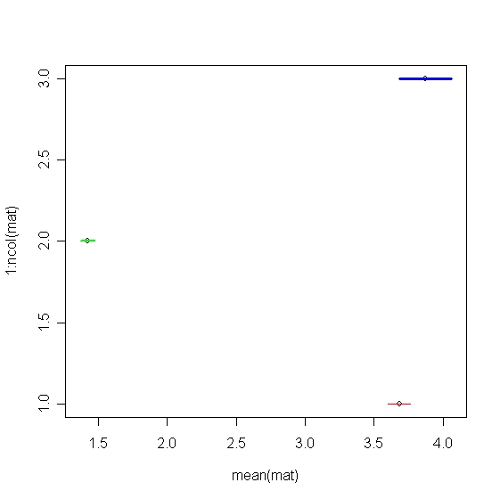