Lecture 2, Tuesday 8/28
These notes contain only the terminology and main calculations in the lectures. For the associated discussions, please come to lecture.
Random Variable
For the purposes of this class, a random variable $X$ is a real valued function on an outcome space.
$$ X: ~ \Omega \longrightarrow \mathbb{R} $$
A precise definition needs more care, of the same sort that is needed to ensure that the probability function $P$ is defined on a sufficiently rich class of sets.
Random variables are often denoted by late letters in the alphabet, such as $X$ and $Y$.
For $S \subseteq R$, the event $\{\omega: X(\omega) \in S\}$ is written as "$X \in S$". For example, we write $P(X > 10)$ or $P(\vert X - 5\vert \le 2)$ etc.
The possible values of $X$ are the real numbers $x$ such that $X(\omega) = x$ for some $\omega \in \Omega$. The set of possible values is also called the range of $X$.
Distribution
Informally, the probability distribution of a random variable $X$ is the set of all possible values of $X$ and any way of specifying how probability is distributed over those values.
Exactly how this is done depends on the range of $X$.
Discrete Distribution
If the possible values of $X$ form a discrete set $x_1, x_2, \ldots$, then the distribution of $X$ and can be specified by a probability mass function that puts a "mass" of $P(X = x_i)$ on the value $x_i$.
Note that $$ \sum_{i=1}^\infty P(X = x_i) ~ = ~ 1 $$
Probabilities can be calculated by using the addition rule.
$$ P(X \in S) ~ = ~ \sum_{\{i: x_i \in S\}} P(X = x_i) $$
For example, if $X$ is a positive integer valued random variable, then
$$ P(X > 10) ~ = ~ \sum_{i=11}^\infty P(X = i) $$ and $$ P(\vert X - 5 \vert \le 2) ~ = ~ \sum_{i=3}^7 P(X = i) $$
Probability Histogram
It is useful to visualize discrete distributions as probability histograms. Here is the distribution table of a random variable $X$.
| $~~~~~~~~~~~~~~~~ i$ | 1 | 2 | 3 | 4 | 5 |
|---|---|---|---|---|---|
| $P(X=i)$ | 0.1 | 0.2 | 0.25 | 0.25 | 0.2 |
And here is the probability histogram of $X$. The probability of the event "$X$ is a prime number" is colored gold.
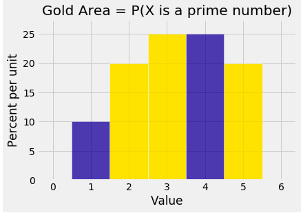
For what follows, it is important to note that histograms represent probabilities by areas. The probability $P(X \text{ is prime})$ is the total area of the gold bars. The total area of all the bars is 1.
Density
A random variable $X$ has probability density function $f$ if
$f$ is a non-negative function on $\mathbb{R}$
$\int_{-\infty}^\infty f(x)dx = 1$
For all $a < b$, $P(a < X \le b) = \int_a^b f(x)dx$
That is, probabilities of events determined by $X$ are areas under the curve $f$.
See the Prob 140 textbook for an example and for the meaning of density.
Cumulative Distribution Function
Another way of specifying the distribution of a random variable is the cumulative distribution function (cdf).
The cdf of a random variable $X$ is the function $F$ from $\mathbb{R}$ to $[0, 1]$ defined by
$$ F(x) ~ = ~ P(X \le x), ~~~ -\infty < x < \infty $$
Therefore for all $a < b$, $$ P(a < X \le b) ~ = ~ F(b) - F(a) $$
Every cdf starts off at 0, is non-decreasing, and ends up at 1. Formally,
$$ \lim_{x \to -\infty} F(x) = 0, ~~~~~ F(x) \le F(y) ~ \text{ for } x < y, ~~~~~ \lim_{x \to \infty} F(x) = 1 $$
If $X$ is discrete, then for all $x$ $$ F(x) ~ = ~ \sum_{s \le x} P(X = s) $$
The discrete random variable $X$ in our earlier example has distribution table
| $~~~~~~~~~~~~~~~~ i$ | 1 | 2 | 3 | 4 | 5 |
|---|---|---|---|---|---|
| $P(X=i)$ | 0.1 | 0.2 | 0.25 | 0.25 | 0.2 |
and hence its distribution function has the graph shown below.
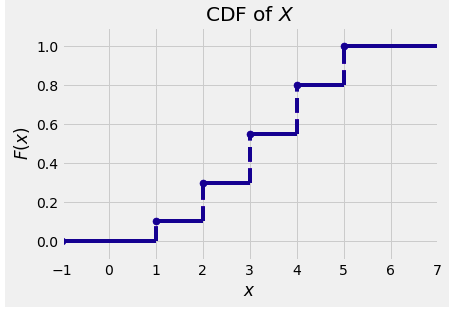
The graph shows a step function with jumps at the possible values of $X$. The size of the jump at $x$ is equal to $P(X = x)$.
If $X$ has density $f$, then by the Fundamental Theorem of calculus, for all $x$
$$ F(x) = \int_{-\infty}^x f(s)ds ~~~~~ \text{ and } ~~~~~ f(x) = \frac{d}{dx}F(x) $$
Bernoulli $(p)$
For a fixed $p \in (0, 1)$, the random variable $X$ has the Bernoulli $(p)$ distribution if
$$ P(X = 0) = 1-p ~~~~~ \text{ and } ~~~~~ P(X = 1) = p $$
We will frequently use the notation $q$ for $1-p$.
Uniform on $\{1, 2, 3, \ldots, n\}$
$X$ has the uniform distribution on the integers 1 through $n$ if $P(X = i) = 1/n$ for $1 \le i \le n$. The probability histogram of $X$ is flat, and for all subsets $S$ of $\{1, 2, \ldots, n\}$, $P(X \in S)$ is the proportion $\#(S)/n$.
Uniform on $(0, 1)$
This one is of fundamental importance, for reasons that will become clear as the course progresses.
The random variable $U$ is uniform on the unit interval if its density is flat over that interval and zero everywhere else:
$$ f_U(u) = \begin{cases} 1 ~~~~~~ \text{if } 0 < u < 1 \\ 0 ~~~~~~ \text{otherwise} \end{cases} $$
The density is flat, so $P(a < U \le b)$ is the area of a rectangle with base $(b-a)$ and height 1. So $P(a < U \le b) = b-a$ and the cdf is linear between 0 and 1:
$$ F_U(u) = \begin{cases} 0 ~~~ \text{if } u \le 0 \\ u ~~~ \text{if } 0 < u < 1 \\ 1 ~~~ \text{if } u \ge 1 \end{cases} $$
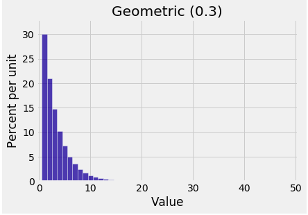
Geometric $(p)$ on $\{1, 2, 3, \ldots \}$
A coin that lands heads with probability $p$ is tossed till H appears. Let $X$ be the number of tosses required. Then $X$ has the geometric $(p)$ distribution on $\{1, 2, 3, \ldots \}$ given by
$$ P(X = k) = q^{k-1}p, ~~~ k \ge 1 $$
Here $q = 1-p$. The probabilities are the terms in a geometric series. You should check that they add up to 1.
The tail probabilities are $$ P(X > k) = P(\text{first } k \text{ tosses are T}) = q^k $$
This can be calculated more laboriously as $$ P(X > k) ~ = ~ \sum_{j=k+1}^\infty q^{j-1}p ~ = ~ q^kp \sum_{i=0}^\infty q^i ~ = ~ q^kp \cdot \frac{1}{1-q} = q^k $$
In many texts the definition of the geometric distribution is slightly different. The random variable $Y$ is the number of tails before the first head. Then $Y = X-1$ and has the geometric $(p)$ distribution on $\{0, 1, 2, \ldots\}$ given by
$$ P(Y = j) = q^jp, ~~~ j \ge 0 $$
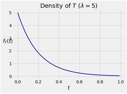
Exponential $(\lambda )$
A random variable $T$ has the exponential distribution with parameter $\lambda$ if the density of $T$ is given by
$$ f_T(t) ~ = \lambda e^{-\lambda t}, ~~~ t \ge 0 $$
At $t > 0$, the cdf of $T$ is $$ F_T(t) ~ = ~ \int_0^t \lambda e^{-\lambda s} ds = 1 - e^{-\lambda t} $$
Since $T$ is often thought of as a lifetime, the tail probability $P(T > t)$ is the chance of survival beyond time $t$. The survival function of $T$ is
$$ S_T(t) ~ = ~ P(T > t) ~ = ~ 1 - F_T(t) ~ = ~ e^{-\lambda t} $$
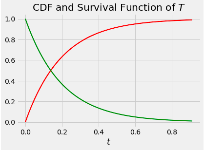
The median of the distribution is the value of $t$ where the two curves intersect. If $m$ is the median, then $e^{-\lambda m} = 0.5$ and so
$$ m ~ = ~ \frac{\log(2)}{\lambda} $$
Memoryless Property
Let $s$ and $t$ be positive. Then $$ P(T > t+s \mid T > t) = \frac{P(T > t+s, T > t)}{P(T > t)} = \frac{P(T > t+s)}{P(T > t)} = \frac{e^{-\lambda(t+s)}}{e^{-\lambda t}} = e^{-\lambda s} = P(T > s) $$
The Rate
The parameter $\lambda$ is called the rate of the distribution. To see why, let $\Delta_t$ be a tiny increment of time and use the memoryless property:
$$ P(T \le t + \Delta_t \mid T > t) ~ = ~ 1 - e^{-\lambda \Delta_t} ~ \sim ~ \lambda \Delta_t ~~~~~ \mbox{because } \Delta_t \mbox{ is small} $$
So $\lambda$ is the instantaneous death rate:
$$ \lambda ~ \sim ~ \frac{P(T \le t+\Delta_t \mid T > t)}{\Delta_t} $$