Measure Theory Basics
\[ \newcommand{\cB}{\mathcal{B}} \newcommand{\cF}{\mathcal{F}} \newcommand{\cN}{\mathcal{N}} \newcommand{\cX}{\mathcal{X}} \newcommand{\EE}{\mathbb{E}} \newcommand{\PP}{\mathbb{P}} \newcommand{\RR}{\mathbb{R}} \newcommand{\td}{\,\textrm{d}} \]
Measure theory: a rigorous grounding for probability
Measure theory is an area of mathematics concerned with measuring the “size” of subsets of a certain set. Soon after it was developed in the the early twentieth century, the great Soviet mathematician Kolmogorov realized it could be applied to give a rigorous grounding to probability theory, it was a major advance in understanding and resolving certain paradoxes in probability theory. David Aldous gives a nice discussion of this history.
This is not a course on measure-theoretic probability and we will not rigorously develop the subject. However, it will be useful to draw on some of the basics of measure theory, to simplify our notation throughout the course and to clarify certain concepts around integration and conditioning. Homework 0 illustrates some of the interesting aspects of measure theory and why it is useful.
Measures
Given a set \(\cX\), a measure\(\mu\) is a certain kind of function mapping “nice enough” subsets \(A \subseteq \cX\) to non-negative numbers \(\mu(A) \in [0,\infty]\).
Example 1 (Counting measure): If \(\cX\) is countable, e.g. \(\cX = \mathbb{Z}\), then a natural measure is the counting measure \(\#(A)\), which simply counts the number of points in a subset \(A\). That is, \(\#(\{0,1\}) = 2\), and \(\#(\{2,4,6,8,\ldots\}) = \infty\) .
Example 2 (Lebesgue measure): If \(\cX = \RR^n\) for some integer \(n\), a natural measure is the Lebesgue measure \(\lambda(A)\), which returns the volume of a subset \(A\). Roughly speaking, we can write
\[ \lambda(A) = \int \cdots \int_A \td x_1\td x_2\cdots \td x_n. \]
Example 3 (Gaussian measure): Now taking \(\cX = \RR\), we might instead want to define the “size” of a set as the probability that a standard Gaussian random variable \(Z \sim \cN(0,1)\) is observed to be in the set \(A\). That is, we can define the measure:
\[ P_Z(A) = \PP(Z \in A) = \int_A \phi(x)\td x, \quad \text{ where } \;\phi(x) = \frac{1}{\sqrt{2\pi}} e^{-x^2/2} \]
is the probability density function of \(Z\).
As it turns out, it is not so obvious how to define what exactly we mean by the right-hand side of the previous two equations; in fact, it is not even possible to define the volume of every subset \(A \in \mathbb{R}\). In Homework 0, Problem 3, you will use the axiom of choice to construct pathological subsets (so-called non-measurable sets) to which we cannot sensibly assign any volume.
One of the original motivations for measure theory was to provide a framework for excluding these pathological sets and rigorously defining integrals over the other, nicer sets. In general, the domain of a measure is not all subsets of \(\cX\) (called the power set and notated \(2^{\cX}\)), but rather a collection of nice subsets \(\cF \subseteq 2^{\cX}\).
Formally, the collection \(\cF\) must be a \(\sigma\)-field, meaning that it satisfies certain closure properties. We say \(\cF\) is a \(\sigma\)-field (or \(\sigma\)-algebra) if
The full set \(\cX\) is in \(\cF\).
If \(A\) is in \(\cF\) then its complement \(\cX \setminus A\) is also in \(\cF\) (i.e., \(\cF\) is closed under complementation)
If \(A_1,A_2,\ldots \in \cF\) then \(\bigcup_{i=1}^\infty A_i\) is also in \(\cF\) (i.e. \(\cF\) is closed under countable unions)
Note: The details of this definition are not important for purposes of this course.
Example: If \(\cX\) is countable we can take \(\cF\) to be the entire power set.
Example: If \(\cX = \mathbb{R}^n\) we will typically use the Borel \(\sigma\)-field \(\cB\), defined as the smallest \(\sigma\)-field that includes all open rectangles \((a_1,b_1)\times (a_2,b_2) \times \cdots \times (a_n, b_n)\), where \(a_i < b_i\) for all \(i\). That is, we start with the open rectangles and recursively apply the closure properties to obtain a very large collection of sets, which informally we can think of as containing all non-pathological subsets of \(\mathbb{R}^n\).
We are now ready to define a measure. We call a pair of a set \(\cX\) and an associated \(\sigma\)-field \(\cF \subseteq 2^{\cX}\) a measurable space. Given a measurable space \((\cX, \cF)\), a measure is a function \(\mu: \cF \to \mathbb{R}\) satisfying three properties:
Non-negativity: \(\mu(A) \geq 0\) for all \(A\in \cF\).
Empty set maps to zero: \(\mu(\emptyset) = 0\)
Countable additivity: If \(A_1,A_2,\ldots\in \cF\) are all disjoint, then
\[ \mu\left(\bigcup_{i=1}^\infty A_i\right) = \sum_{i=1}^\infty \mu(A_i) \]
If \(\mu\) is a measure on \((\cX, \cF)\) we call \((\cX, \cF, \mu)\) a measure space.
In the special case \(\mu(\cX) = 1\), we call \(\mu\) a probability measure and \((\cX, \cF, \mu)\) is called a probability space.
Integrals
One very nice thing about measures is that they let us define integrals of (nice enough) real-valued functions on \(\cX\) with respect to the measure \(\mu\), meaning the integral is “weighted” in a way that assigns total weight \(\mu(A)\) to each set \(A\). We will use the notation \(\int f(x)\,\td\mu(x)\), or just \(\int f \td\mu\).
To construct this integral, we begin by defining it for indicator functions, and then extend to more general functions by linearity and limits, in a few steps:
First, for an indicator function \(1_A(x) = 1\{x \in A\}\) of a set \(A \in \cF\), it is straightforward to define the integral as \(\int 1_A \td\mu = \mu(A)\) (note if \(A \notin \cF\) this does not work, but we are only defining the integral for a class of “nice” functions determined by our \(\sigma\)-field)
Next, consider a simple function \(f(x) = \sum_{i=1}^\infty c_i 1_{A_i}(x)\), with all \(c_i \geq 0\) and \(A_i \in \cF\). Because the integral should be linear, we should have
\[ \int f\td\mu = \sum_{i=1}^\infty c_i \int 1_{A_i}\td\mu = \sum_{i=1}^\infty c_i \mu(A_i) \]
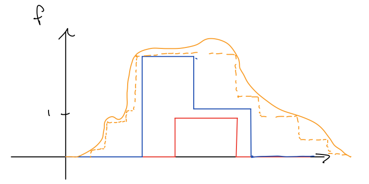
Third, we can extend to all sufficiently nice non-negative functions by approximating them from below with a series of simple functions:
\[ \int f\td\mu = \lim_{i=1}^\infty \int f_i\td\mu. \]
This idea is illustrated in the picture below:
Finally, we can write any real-valued function as the sum of its positive and negative parts, \(f(x) = f^+(x) - f^-(x)\), where \(f^+(x) = \max\{f(x), 0\}\) and \(f^-(x) = \max\{-f(x), 0\}\). Then both \(f^+\) and \(f^-\) have non-negative (possibly infinite) integrals. Then we simply take
\[ \int f\td\mu = \int f^+\td\mu - \int f^-\td\mu \in [-\infty, \infty], \]
calling the difference undefined if the integrals of both \(f^+\) and \(f^-\) are infinite.
As a result, we have \(\int f\td\mu\) for any function \(f\) whose positive and negative parts can both be approximated from below by simple functions. Note that we have left out some important details in this presentation (for example we have not characterized which functions \(f\) are nice enough to be approximated well by simple functions) but these details are unimportant for this class. The important thing to know is that to any measure \(\mu\) there corresponds a well-defined integral \(\int \cdot \td\mu\), which behaves as we would expect it to.
We can now return to our previous examples of measures and ask what the corresponding integrals are:
Example 1, continued (Counting measure): An integral with respect to \(\#\) just adds up all the values of \(f(x)\):
\[ \int f\td\# = \sum_{x\in \cX} f(x) \]
Example 2, continued (Lebesgue measure): An integral with respect to the Lebesgue measure is called a Lebesgue integral, which is essentially just the usual integral you are used to from calculus class:
\[ \int f\td\lambda = \int\cdots \int f(x) \td x_1 \cdots \td x_n. \]
The Lebesgue integral extends the Riemann integral to a more general class of functions, in the sense that if the Riemann integral of \(f\) is defined then the Lebesgue integral is also well defined and the two integrals coincide. But the Lebesgue integral is also well-defined for functions like \(f(x) = 1\{x \in \mathbb{Q}\}\), for which the Riemann integral is not well-defined (Exercise: what is the Lebesgue integral of \(1\{x \in \mathbb{Q}\}\)?)
Example 3, continued (Gaussian measure): Note that \(P_Z(A)\) is defined as the (Lebesgue) integral of \(1_A(x)\phi(x)\). By extension, the integral of \(f\) with respect to \(P_Z\) is the Lebesgue integral of \(f(x) \phi(x)\), which is nothing more than the expectation of \(f(Z)\):
\[ \int f\td P_Z = \int_{-\infty}^\infty f(x) \phi(x) \td x = \EE[f(Z)]. \]
Densities
We have just seen in the last two examples that there is a special relationship between the Lebesgue measure \(\lambda\) on \(\RR\) and the Gaussian measure \(P_Z\), allowing us to evaluate integrals with respect to \(P\) by turning them into integrals with respect to \(\lambda\), namely \(\int f(x)\td P_Z(x) = \int f(x)\phi(x) \td\lambda(x)\).
This is a happy fact, since mathematicians have gone to a lot of trouble figuring out how to calculate integrals with respect to the usual (Lebesgue) measure. Most of the expectations we want to calculate in statistics are integrals with respect to some joint probability measure over random variables, and we certainly wouldn’t want to have to reinvent the wheel of integration every time we want to do calculations with respect to a new random variable.
Note that we can’t turn integrals for every random variable into Lebesgue integrals. If \(Y\) follows a binomial distribution, for example, we can just as well define \(P_Y(A) = \PP(Y \in A)\), but there is no counterpart to \(\phi\) that would let us turn \(P_Y\) integrals into Lebesgue integrals in the same way.
Formally, consider a measurable space \((\cX, \cF)\), with two measures \(P\) and \(\mu\). We say \(P\) is absolutely continuous with respect to \(\mu\) if \(P(A) = 0\) whenever \(\mu(A) = 0\). In notation, we write \(P \ll \mu\).
If \(P \ll \mu\) then, under mild conditions, we can always define a density function \(p:\cX \mapsto [0,\infty)\) such that
\[ P(A) = \int 1_A(x) p(x)\td\mu(x), \quad \text{ for all } A \in \cF, \]
and by extension \(\int f(x)\td P(x) = \int f(x) p(x) \td\mu(x)\).
The function \(p\) is called the density function or Radon-Nikodym derivative of \(P\) with respect to \(\mu\). It is sometimes written using the suggestive notation \(\frac{\td P}{\td\mu}(x)\). Whenever we have a density function we can turn integrals with respect to \(P\) into integrals with respect to \(\mu\) simply by multiplying the integrand by \(p\).
If we do not specify what \(\mu\) is, it is assumed to be the Lebesgue measure; that is, if we say \(P\) is absolutely continuous with no further elaboration, we mean \(P \ll \lambda\).
If \(P\) is a probability measure, we call \(p(x)\) its probability density function (with respect to \(\mu\)). If \(\mu\) is a counting measure, we call \(p(x)\) its probability mass function. These are abbreviated pdf and pmf, respectively.
Probability spaces and random variables
A typical statistics problem involves many, random variables of various types (e.g. some discrete and some continuous random variables), some of which may be functions of others. The overall joint distribution is defined implicitly by specifying the variables’ relationships to one another, or giving some sequence of rules for how they are all generated. We will want to ask about probabilities of events that involve functions of multiple random variables, e.g. a natural question to ask in a simple variance estimation problem with i.i.d. random variables \(X_1,\ldots,X_n\) might be “what is the probability that \(\left|\frac{1}{n-1}\sum_{i=1}^n \left(X_i - \overline X\right)^2 - \sigma^2\right| < \delta\) ?”
The notation in the previous section doesn’t allow us to ask questions like this without, e.g., massaging the above event into the set of \((X_1,\ldots,X_n)\) vectors for which the event would hold. This would become even more difficult in more complicated setups.
Instead of trying to work directly with the measure corresponding to the joint distribution of all of the random variables involved, it can be convenient to instead think of the variables as all being functions of some abstract “outcome” \(\omega\) that encompasses all of the randomness in the problem. We introduce an abstract probability space \((\Omega, \cF, \PP)\) where
\(\omega \in \Omega\) is called an outcome,
\(A \in \cF\) is called an event,
\(\PP(A)\) is called the probability of \(A\).
Then a random variable is any (nice enough) function \(X:\; \Omega \to \cX\). We say \(X\) has distribution \(P\), and write \(X \sim P\), if
\[ \PP(X \in B) = \PP(\{\omega:\; X(\omega) \in B\}) = P(B). \]We say the real-valued random variable \(X\) is continuous if its distribution is absolutely continuous (with respect to the Lebesgue meaure). If \(X\) is a random variable, then \(f(X)\) is also a random variable for any (nice enough) function \(f\).
Likewise, the expectation of a random variable is defined as an integral with respect to \(\PP\):
\[ \EE[X] = \int X(\omega) \td\PP(\omega), \quad \text{ and } \quad \EE[f(X,Y)] = \int f(X(\omega), Y(\omega)) \td\PP(\omega). \]
Usually, to do real calculations we will eventually boil \(\PP\) or \(\EE\) into a composition of integrals and/or sums.
Conditional probability
While it is beyond the scope of this course, measure theory also allows us to patch the definition of conditional probability and conditional expectation. Given two events \(A\) and \(B\), if \(\PP(B) > 0\), we can unproblematically define the conditional probability of \(A\) given \(B\) as \(\PP(A \mid B) = \PP(A \cap B) / \PP(B)\), but this definition obviously fails when \(\PP(B) = 0\).
Generally speaking, we cannot necessarily define \(\PP(A \mid B)\) for measure zero events \(B\) (Homework 0 includes a problem illustrating the inherent ambiguity of this definition). But, for example, if \(X\) and \(Y\) are both continuous random variables with some dependence between them we would like to be able to discuss, e.g., the distribution or expectation of \(Y\) given that \(X\) takes on some specific value \(x\). We can do this by defining the conditional expectation \(\EE(Y \mid X)\) as a random variable \(g(X)\), which has the property \(\EE[(Y - g(X)) 1_A(X)] = 0\) for all (nice) subsets \(A\). By evaluating this function \(g\) at \(x\) we can answer the question we asked earlier. However, note this explanation is informal and brushes many important points under the rug; for a more complete explanation, take Stat 205A.
Having defined the conditional expectation, we can also ask about the conditional distribution of \(Y\) by evaluating the conditional expectation on new random variables defined with indicator functions: \(\PP(Y \in A \mid X) = \EE[1_A(Y) \mid X]\) .
More definitions
Finally, this section includes some scattered definitions to remind you of a few more useful definitions which you likely have already seen in your previous probability courses.
If \(\PP(A) = 1\), we say \(A\) occurs almost surely.
The variance of a random variable \(X\) is \(\textrm{Var}(X) = \EE[X^2] - \EE [X]\)
See Keener Ch. 1 for more on probability.