This is a multi-week project where pieces of is could be broken off and presented as homework assignments.

Outline of Scientific Context

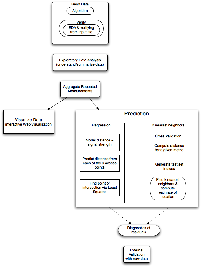
This project involves trying to predict the location of a wireless device based on the signal strength received at 6 different fixed access points (routers) within a building. It is of interest as GPS does not work well within buildings and the hope is to get more accurate predictions. The experiment associated with this particular data set also includes orientation, i.e. the direction the person holding the device is facing as this is expected to have a significant impact on signal strength when the person is between the device and an access point.

There are two sets of data - training (offline) data and test (online) data. There are approximately 1 million records in the offline data. There are many repeated measurements and significant complexity to visualizing the volume of data wrt the small number of factors. This clearly has a spatial component.

We (Deb and I) worked on this in 2007 (?). There is now a new data set and a different building plan.

Computational Topics Covered

Learning Objectives

Prerequisite Computational Topics

Essentials of string manipulation (without regular expressins). Eventhough one can use regular expressions, simple string manipulation will suffice.
data structures
graphics
writing functions

Prerequisite Statistical Background

None for the k-nearest neighbor approach. This can be taught as part of the activity.

If one uses the regression approaach, then of course the students should know enough about regression to be able to fit a model and understand what it means, to be able to use transformed variables and do diagnostics.

How to integrate into a class

This is a multi-week project. The data input can be covered separately, early on, where the focus would be on getting the data into a format for analysis. One can also give the students the data and have them explore it and produce interesting graphical displays and summaries when discussing graphics early in the course (after they have seen data frames and subsetting).

Level/Target Student

The target a udience is an advanced undergraduate/first year graduate student. The graduate student audience may delve deeper into the model fitting aspects of the project.

Breakdown of Computational Tasks

Solutions

[Data Access] Reading the data is somewhat complicated because each line is of the form
t=1139692477303;id=00:02:2D:21:0F:33;pos=0.0,0.05,0.0;degree=130.5;00:14:bf:b1:97:8a=-43,2437000000,3;00:0f:a3:39:e1:c0=-52,2462000000,3;00:14:bf:3b:c7:c6=-62,2432000000,3;00:14:bf:b1:97:81=-58,2422000000,3;00:14:bf:b1:97:8d=-62,2442000000,3;00:14:bf:b1:97:90=-57,2427000000,3;00:0f:a3:39:e0:4b=-79,2462000000,3;00:0f:a3:39:e2:10=-88,2437000000,3;00:0f:a3:39:dd:cd=-64,2412000000,3;02:64:fb:68:52:e6=-87,2447000000,1;02:00:42:55:31:00=-85,2457000000,1 t=1139692477555;id=00:02:2D:21:0F:33;pos=0.0,0.05,0.0;degree=130.5;00:14:bf:b1:97:8a=-43,2437000000,3;00:14:bf:b1:97:8a=-43,2437000000,3;00:0f:a3:39:e1:c0=-52,2462000000,3;00:14:bf:b1:97:90=-57,2427000000,3;00:14:bf:b1:97:8d=-64,2442000000,3;00:0f:a3:39:e0:4b=-77,2462000000,3;00:0f:a3:39:dd:cd=-62,2412000000,3;02:00:42:55:31:00=-85,2457000000,1;02:64:fb:68:52:e6=-88,2447000000,1
So we have to get the time stamp, then the MAC of the hand-held device, then the position and orientiation. Then we have a ragged array of mac=triple.
This is one of those formats that requires some thought to identify the pattern that makes the code simple to read into an R data structure. One also has to think carefully about the right data format.
The auxiliary data giving the locations of the access points can be given as a CSV file or an RDA file.

[EDA] Given the data, the students explore it.

Compute the number of repeated observations at each location and orientation.
Find the number of devices that were detected and the different types. One can even look up the MAC address to find the type of device, i.e. the vendor and model.
Look at the times the measurements were taken.
Look at the distribution of the signal strengths
Look at signal strength as a function of (Euclidean) distance.

Students need to collapse the repeated measurements to compute average/median for each location and orientation for each access point.

One significant activity is to come up with graphical displays of this data that summarize it effectively. (Or even create interactive plots where a plot of, say, the densities of the signal strengths from a particular point to each of the 6 access points, is displayed in one "panel" when the viewer mouses over that point in the building layout.)

[Prediction]
In this stage, we develop a predictor for the location of the hand-held device based on the signal strength between the access points and a new device. There are two approaches students might explore.

k Nearest Neighbors

Here we predict the location of an observation based on its 6 signal strengths - 1 to each of the access points. We find the k observations in our observed data sets based on Signal Strength distances. Then we take an average of their locations to get our prediction.

We use cross-validation to determine k, the choice of metric, and how to weight the neighboring locations (e.g. uniform weights or weights inversely proportional to distance).
This again (like the Spam problem) raises computational issues regarding computing the distance matrix and k-nearest neighbors generally. Cross-validation is introduced.

Regression
This version exploits the existence of a relationship between signal strength and distance. We develop regression models to determine the distance of a point based on its signal strength to an access point. For each observation, we end up with an estimate of distance to each of the 6 access points. If there were no errors, we would only need two of these and we could find the point of intersection of the circles centered at the two access points with the predicted radii. However, there are errors and so we use least squares to "triangulate" a location.
There are all sorts of issues with standard errors of the different estimates and weighting the predictions, i.e. variance of the distance estimates probably increas with distance (i.e. less accurate the further away we are). We could use tehse in a weighted least squares to solve the "point of intersection".

[EDA] Diagnose the predictions, trying to understand why it does better in some places than others and see if we can modify the approach to improve the results.

Validation of the predictor based on an entirely new data set.
[EDA] Given the data, the students explore it.

Compute the number of repeated observations at each location and orientation.
Find the number of devices that were detected and the different types. One can even look up the MAC address to find the type of device, i.e. the vendor and model.
Look at the times the measurements were taken.
Look at the distribution of the signal strengths
Look at signal strength as a function of (Euclidean) distance.

Students need to collapse the repeated measurements to compute average/median for each location and orientation for each access point.

One significant activity is to come up with graphical displays of this data that summarize it effectively. (Or even create interactive plots where a plot of, say, the densities of the signal strengths from a particular point to each of the 6 access points, is displayed in one "panel" when the viewer mouses over that point in the building layout.)

[Prediction]
In this stage, we develop a predictor for the location of the hand-held device based on the signal strength between the access points and a new device. There are two approaches students might explore.

k Nearest Neighbors

Here we predict the location of an observation based on its 6 signal strengths - 1 to each of the access points. We find the k observations in our observed data sets based on Signal Strength distances. Then we take an average of their locations to get our prediction.

We use cross-validation to determine k, the choice of metric, and how to weight the neighboring locations (e.g. uniform weights or weights inversely proportional to distance).
This again (like the Spam problem) raises computational issues regarding computing the distance matrix and k-nearest neighbors generally. Cross-validation is introduced.

Regression
This version exploits the existence of a relationship between signal strength and distance. We develop regression models to determine the distance of a point based on its signal strength to an access point. For each observation, we end up with an estimate of distance to each of the 6 access points. If there were no errors, we would only need two of these and we could find the point of intersection of the circles centered at the two access points with the predicted radii. However, there are errors and so we use least squares to "triangulate" a location.
There are all sorts of issues with standard errors of the different estimates and weighting the predictions, i.e. variance of the distance estimates probably increas with distance (i.e. less accurate the further away we are). We could use tehse in a weighted least squares to solve the "point of intersection".

[EDA] Diagnose the predictions, trying to understand why it does better in some places than others and see if we can modify the approach to improve the results.

Validation of the predictor based on an entirely new data set.
Students need to collapse the repeated measurements to compute average/median for each location and orientation for each access point.

One significant activity is to come up with graphical displays of this data that summarize it effectively. (Or even create interactive plots where a plot of, say, the densities of the signal strengths from a particular point to each of the 6 access points, is displayed in one "panel" when the viewer mouses over that point in the building layout.)

[Prediction]
In this stage, we develop a predictor for the location of the hand-held device based on the signal strength between the access points and a new device. There are two approaches students might explore.

k Nearest Neighbors

Here we predict the location of an observation based on its 6 signal strengths - 1 to each of the access points. We find the k observations in our observed data sets based on Signal Strength distances. Then we take an average of their locations to get our prediction.

We use cross-validation to determine k, the choice of metric, and how to weight the neighboring locations (e.g. uniform weights or weights inversely proportional to distance).
This again (like the Spam problem) raises computational issues regarding computing the distance matrix and k-nearest neighbors generally. Cross-validation is introduced.

Regression
This version exploits the existence of a relationship between signal strength and distance. We develop regression models to determine the distance of a point based on its signal strength to an access point. For each observation, we end up with an estimate of distance to each of the 6 access points. If there were no errors, we would only need two of these and we could find the point of intersection of the circles centered at the two access points with the predicted radii. However, there are errors and so we use least squares to "triangulate" a location.
There are all sorts of issues with standard errors of the different estimates and weighting the predictions, i.e. variance of the distance estimates probably increas with distance (i.e. less accurate the further away we are). We could use tehse in a weighted least squares to solve the "point of intersection".

[EDA] Diagnose the predictions, trying to understand why it does better in some places than others and see if we can modify the approach to improve the results.

Validation of the predictor based on an entirely new data set.
One significant activity is to come up with graphical displays of this data that summarize it effectively. (Or even create interactive plots where a plot of, say, the densities of the signal strengths from a particular point to each of the 6 access points, is displayed in one "panel" when the viewer mouses over that point in the building layout.)

[Prediction]
In this stage, we develop a predictor for the location of the hand-held device based on the signal strength between the access points and a new device. There are two approaches students might explore.

k Nearest Neighbors

Here we predict the location of an observation based on its 6 signal strengths - 1 to each of the access points. We find the k observations in our observed data sets based on Signal Strength distances. Then we take an average of their locations to get our prediction.

We use cross-validation to determine k, the choice of metric, and how to weight the neighboring locations (e.g. uniform weights or weights inversely proportional to distance).
This again (like the Spam problem) raises computational issues regarding computing the distance matrix and k-nearest neighbors generally. Cross-validation is introduced.

Regression
This version exploits the existence of a relationship between signal strength and distance. We develop regression models to determine the distance of a point based on its signal strength to an access point. For each observation, we end up with an estimate of distance to each of the 6 access points. If there were no errors, we would only need two of these and we could find the point of intersection of the circles centered at the two access points with the predicted radii. However, there are errors and so we use least squares to "triangulate" a location.
There are all sorts of issues with standard errors of the different estimates and weighting the predictions, i.e. variance of the distance estimates probably increas with distance (i.e. less accurate the further away we are). We could use tehse in a weighted least squares to solve the "point of intersection".

[EDA] Diagnose the predictions, trying to understand why it does better in some places than others and see if we can modify the approach to improve the results.

Validation of the predictor based on an entirely new data set.
[Prediction]
In this stage, we develop a predictor for the location of the hand-held device based on the signal strength between the access points and a new device. There are two approaches students might explore.

k Nearest Neighbors

Here we predict the location of an observation based on its 6 signal strengths - 1 to each of the access points. We find the k observations in our observed data sets based on Signal Strength distances. Then we take an average of their locations to get our prediction.

We use cross-validation to determine k, the choice of metric, and how to weight the neighboring locations (e.g. uniform weights or weights inversely proportional to distance).
This again (like the Spam problem) raises computational issues regarding computing the distance matrix and k-nearest neighbors generally. Cross-validation is introduced.

Regression
This version exploits the existence of a relationship between signal strength and distance. We develop regression models to determine the distance of a point based on its signal strength to an access point. For each observation, we end up with an estimate of distance to each of the 6 access points. If there were no errors, we would only need two of these and we could find the point of intersection of the circles centered at the two access points with the predicted radii. However, there are errors and so we use least squares to "triangulate" a location.
There are all sorts of issues with standard errors of the different estimates and weighting the predictions, i.e. variance of the distance estimates probably increas with distance (i.e. less accurate the further away we are). We could use tehse in a weighted least squares to solve the "point of intersection".

[EDA] Diagnose the predictions, trying to understand why it does better in some places than others and see if we can modify the approach to improve the results.

Validation of the predictor based on an entirely new data set.: In this stage, we develop a predictor for the location of the hand-held device based on the signal strength between the access points and a new device. There are two approaches students might explore.

k Nearest Neighbors

Here we predict the location of an observation based on its 6 signal strengths - 1 to each of the access points. We find the k observations in our observed data sets based on Signal Strength distances. Then we take an average of their locations to get our prediction.

We use cross-validation to determine k, the choice of metric, and how to weight the neighboring locations (e.g. uniform weights or weights inversely proportional to distance).
This again (like the Spam problem) raises computational issues regarding computing the distance matrix and k-nearest neighbors generally. Cross-validation is introduced.

Regression
This version exploits the existence of a relationship between signal strength and distance. We develop regression models to determine the distance of a point based on its signal strength to an access point. For each observation, we end up with an estimate of distance to each of the 6 access points. If there were no errors, we would only need two of these and we could find the point of intersection of the circles centered at the two access points with the predicted radii. However, there are errors and so we use least squares to "triangulate" a location.
There are all sorts of issues with standard errors of the different estimates and weighting the predictions, i.e. variance of the distance estimates probably increas with distance (i.e. less accurate the further away we are). We could use tehse in a weighted least squares to solve the "point of intersection".
[EDA] Diagnose the predictions, trying to understand why it does better in some places than others and see if we can modify the approach to improve the results.

Validation of the predictor based on an entirely new data set.
Validation of the predictor based on an entirely new data set.

Cautionary Notes

There can be confusion computing distances in the space of signal strength and distance in the physcial space of the building. The k-nearest neighbors works on the signal strengths and distance between two observations is the sum over access points of the squared differences between the signal strengths to the same access point.

Geolocation

Type of Activity

Outline of Scientific Context

Computational Topics Covered

Learning Objectives

Prerequisite Computational Topics

Essentials of string manipulation (without regular expressins). Eventhough one can use regular expressions, simple string manipulation will suffice.
data structures
graphics
writing functions

Prerequisite Statistical Background

How to integrate into a class

Level/Target Student

Breakdown of Computational Tasks

Solutions

Cautionary Notes

Extensions

Different Directions

Grading Suggestions

Similar Activities/Assignments

Geolocation

Type of Activity

Outline of Scientific Context

Computational Topics Covered

Learning Objectives

Prerequisite Computational Topics

Essentials of string manipulation (without regular expressins). Eventhough one can use regular expressions, simple string manipulation will suffice. data structures graphics writing functions

Prerequisite Statistical Background

How to integrate into a class

Level/Target Student

Breakdown of Computational Tasks

Solutions

Cautionary Notes

Extensions

Different Directions

Grading Suggestions

Similar Activities/Assignments

Essentials of string manipulation (without regular expressins). Eventhough one can use regular expressions, simple string manipulation will suffice.
data structures
graphics
writing functions