Linear Regression
1 Linear Regression
Linear regression is a very popular procedure for modeling the value of one
variable on the value(s) of one or more other variables. The variable that
we're trying to model or predict is known as the dependent variable, and the
variables that we use to make predictions are known as independent variables,
or covariates. Linear regression makes the assumption that the changes in the
dependent variable can be modeled as a monotonic linear function of the
independent variables; that is, we assume that a change of a certain amount
in the independent variables will result in a change in the dependent variable,
and the amount of change in the dependent variable is constant across the range
of the independent variables. As a simple example, suppose we're interested in
the relationship between the horsepower of a car (the independent variable) and
the miles per gallon of gas (MPG) of the car. When we fit a linear regression
model, we're saying that a change of one horsepower will have the same effect on
the MPG regardless of the value of horsepower that we're changing. In other words,
a linear regression model would assume that if we had a car with 100 horsepower,
and compared it to a car with 101 horsepower, we'd see the same difference in
MPG as if we had a car with 300 horsepower and compared it to a car with 301
horsepower. Relationships like this often hold for a limited range of independent
variable values, but the linear regression model assumes that it applies for the
entire range of the independent variables.
Even with these limitations, linear regression has proven itself to be a very
valuable tool for modeling, and it's widely used in many branches of research.
There are also a variety of diagnostic measures, both numerical and graphical,
that can help us to determine whether the regression is doing a good job, so
it's not unreasonable that many people use linear regression as their first
tool when trying to model a variable of interest.
2 The lm command
The lm command uses the model-based formula interface that we've already
seen in the context of lattice graphics. The dependent variable is placed on the
left-hand side of the tilde (~), and the independent variables are placed on
the right-hand side, joined together with plus signs (+). When you want
to use all the variables in a data frame (except for the dependent variable) as
independent variables, you can use a period (.) for the right-hand side of
the equation.
These models correspond to a mathematical model that looks like this:
|
yi = b0 + b1 x1 + b2 x2 + ... + bp xp + ei for i=1,...,n |
| (1) |
The bs represent coefficients that measure how much the dependent variable
changes for each unit of change in the independent variable, and are often refered
to as the slopes. The term b0 is often known as the intercept. (To omit
the intercept in a formula in R, insert the term -1.) The e's represent
the part of the observed dependent variable that can't be explained by the regression
model, and in order to do hypothesis testing, we assume that these errors follow
a normal distribution. For each term in the model, we test the hypothesis that the
b corresponding to that term is equal to 0, against the alternative that
the b is different from 0.
To illustrate the use of the lm command, we'll construct a regression model
to predict the level of Alcohol in the wine data set, using several
of the other variables as independent variables. First, we'll run lm to
create an lm object containing all the information about the regression:
> wine.lm = lm(Alcohol~Malic.acid+Alkalinity.ash+Proanthocyanins+Color.intensity+OD.Ratio+Proline,data=wine[-1])
To see a very brief overview of the results, we can simply view the lm object:
> wine.lm

Call:
lm(formula = Alcohol ~ Malic.acid + Alkalinity.ash + Proanthocyanins +     Color.intensity + OD.Ratio + Proline, data = wine[-1])

Coefficients:
    (Intercept)       Malic.acid   Alkalinity.ash  Proanthocyanins
      11.333283         0.114313        -0.032440        -0.129636
Color.intensity         OD.Ratio          Proline
       0.158520         0.225453         0.001136
To get more information about the model, the summary function can be called:
> summary(wine.lm)

Call:
lm(formula = Alcohol ~ Malic.acid + Alkalinity.ash + Proanthocyanins +
    Color.intensity + OD.Ratio + Proline, data = wine[-1])

Residuals:
      Min        1Q    Median        3Q       Max
-1.502326 -0.342254  0.001165  0.330049  1.693639

Coefficients:
                  Estimate Std. Error t value Pr(>|t|)
(Intercept)     11.3332831  0.3943623  28.738  < 2e-16 ***
Malic.acid       0.1143127  0.0397878   2.873  0.00458 **
Alkalinity.ash  -0.0324405  0.0137533  -2.359  0.01947 *
Proanthocyanins -0.1296362  0.0846088  -1.532  0.12732
Color.intensity  0.1585201  0.0231627   6.844 1.32e-10 ***
OD.Ratio         0.2254528  0.0834109   2.703  0.00757 **
Proline          0.0011358  0.0001708   6.651 3.76e-10 ***
---
Signif. codes:  0 '***' 0.001 '**' 0.01 '*' 0.05 '.' 0.1 ' ' 1

Residual standard error: 0.5295 on 171 degrees of freedom
Multiple R-Squared: 0.5889,     Adjusted R-squared: 0.5745
F-statistic: 40.83 on 6 and 171 DF,  p-value: < 2.2e-16
The probability levels in the last column of the bottom table are for testing
the null hypotheses that the slopes for those variables are equal to 0; that is,
we're testing the null hypothesis that changes in the independent variable will
not result in a linear change in the dependent variable. We can see that most
of the variables in the model do seem to have an effect on the dependent variable.
One useful measure of the efficacy of a regression model is the multiple
R-Squared statistic. This essentially measures the squared correlation of
the dependent variable values with the values that the model would predict.
The usual interpretation of this statistic is that it measures the fraction of
variability in the data that is explained by the model, so values approaching 1
mean that the model is very effective. Since adding more variables to a model
will always inflate the R-Squared value, many people prefer
using the adjusted R-Squared value,
which has been adjusted to account for the number of variables included in the model.
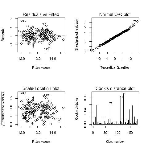
When you pass a model object to the plot function, it will display one or
more plots that the author of the model fitting function felt were appropriate for
studying the effectiveness of the model. For the lm object, four plots are
created by default:
- A plot of residuals versus fitted (predicted) values - The residuals are the part
of the dependent variable that the model couldn't explain, and they are our best
available estimate of the error term from the regression model. They're calculated by
subtracting the predicted value from the actual value of the dependent variable.
Under the usual assumptions for the linear regression model, we don't expect the
variability of the residuals to change over the range of the dependent variable, so
there shouldn't be any discernable pattern to this plot. Note that outliers in the
plot will be labeled by their observation number making it easy to track them down.
-
A normal quantile-quantile plot of the standardized residuals - For the probabilities
we saw in the summary table to be accurate, we have assumed that the errors of the
model follow a normal distribution. Thus, we'd expect a normal quantile-quantile plot
of the residuals to follow a straight line. Deviations from a straight line could mean
that the errors don't follow a normal distribution.
-
A scale-location plot - This plot is similar to the residuals versus fitted values
plot, but it uses the square root of the standardized residuals. Like the first plot,
there should be no discernable pattern to the plot.
-
A Cook's distance plot - Cook's distance is a statistic that tries to identify points
which have more influence than other points. Generally these are points that are
distant from other points in the data, either for the dependent variable or one or more
independent variables. Each observation is represented as a line whose height is
indicative of the value of Cook's distance for that observation. There are no hard and fast
rules for interpreting Cook's distance, but large values (which will be labeled with
their observation numbers) represent points which might require further investigation.
Here are the four plots for the wine.lm object:
3 Using the model object
The design of the R modeling functions makes it very easy to do common tasks, regardless
of the method that was used to model the data. We'll use lm as an example, but
most of these techniques will work for other modeling functions in R.
We've already seen that the plot function will produce useful plots after a
model is fit.
Here are some
of the other functions that are available to work with modeling objects. In each
case, the modeling object is passed to the function as its first argument.
- Coefficients - The coef function will return a vector containing the coefficients
that the model estimated, in this case, the intercept and the slopes for each of the
variables:
> coef(wine.lm)
    (Intercept)      Malic.acid  Alkalinity.ash Proanthocyanins Color.intensity
   11.333283116     0.114312670    -0.032440473    -0.129636226     0.158520051
       OD.Ratio         Proline
    0.225452840     0.001135776
-
Predicted Values - The predict function, called with no additional arguments,
will return
a vector of predicted values for the observations that were used in the modeling process.
To get predicted values for observations not used in building the model, a data frame
containing the values of the observations can be passed to predict through the
newdata= argument. The variables in the data frame passed to predict
must have the same names as the variables used to build the model. For example, to
get a predicted value of Alcohol for a mythical wine, we could use a statement
like this:
> predict(wine.lm,newdata=data.frame(Malic.acid=2.3,Alkalinity.ash=19,
+              Proanthocyanins=1.6,Color.intensity=5.1,OD.Ratio=2,6,Proline=746.9))
[1] 12.88008
-
Residuals - The residuals function will return a vector of the residuals from
a model.
In addition, the summary function, which is usually used to display a printed
summary of a model, often contains useful information. We can see what it contains
by using the names function:
> names(summary(wine.lm))
 [1] "call"          "terms"         "residuals"     "coefficients"
 [5] "aliased"       "sigma"         "df"            "r.squared"
 [9] "adj.r.squared" "fstatistic"    "cov.unscaled"
File translated from
TEX
by
TTH,
version 3.67.
On 25 Apr 2011, 11:23.